Python Basics III

Welcome to Python Basics III — the final Python foundations lecture before numerical methods!

In this notebook, we’ll cover:

1. NumPy Arrays In-Depth — The foundation of scientific computing in Python

2. Advanced Matplotlib — Creating publication-quality figures

3. Vectorization & Performance — Writing fast numerical code

4. Functions as Arguments — Preparing for numerical methods

5. Physics Applications — Putting it all together

By the end of this lecture, you’ll be ready to implement numerical integration, differentiation, and other computational methods.

I. NumPy Arrays In-Depth

NumPy (Numerical Python) is the foundation of scientific computing in Python. The ndarray (n-dimensional array) is its core data structure.

Why NumPy?

• Fast: Operations are implemented in C, much faster than Python loops

• Convenient: Mathematical operations work element-wise

• Memory efficient: Stores data in contiguous memory blocks

• Universal: Used by virtually all scientific Python libraries

import numpy as np
import matplotlib.pyplot as plt

# Check version
print(f"NumPy version: {np.__version__}")

NumPy version: 2.0.2

1. Creating Arrays

There are many ways to create NumPy arrays:

# From a Python list
a = np.array([1, 2, 3, 4, 5], float)
print(f"From list: {a}")
print(f"Type: {type(a)}")
print(f"Shape: {a.shape}")
print(f"Data type: {a.dtype}")

From list: [1. 2. 3. 4. 5.]
Type: <class 'numpy.ndarray'>
Shape: (5,)
Data type: float64

# Zeros, ones, and empty arrays
zeros = np.zeros(5)          # 5 zeros
ones = np.ones(5)            # 5 ones
full = np.full(5, 3.14)      # 5 copies of 3.14

print(f"Zeros: {zeros}")
print(f"Ones: {ones}")
print(f"Full: {full}")

Zeros: [0. 0. 0. 0. 0.]
Ones: [1. 1. 1. 1. 1.]
Full: [3.14 3.14 3.14 3.14 3.14]

# linspace and arange - VERY important for physics!

# linspace: N evenly spaced points between start and end (inclusive)
x1 = np.linspace(0, 10, 5)   # 5 points from 0 to 10
print(f"linspace(0, 10, 5): {x1}")

# arange: points with fixed step (like range, but for floats)
x2 = np.arange(0, 10, 2)     # start=0, stop=10, step=2
print(f"arange(0, 10, 2): {x2}")

### range(0,10)

# Common use: time array for simulations
t = np.linspace(0, 1, 101)   # 0 to 1 second, 101 points (dt = 0.01)
print(f"\nTime array: {t[:10]}... (first 10 of {len(t)} points)")

linspace(0, 10, 5): [ 0.   2.5  5.   7.5 10. ]
arange(0, 10, 2): [0 2 4 6 8]

Time array: [0.   0.01 0.02 0.03 0.04 0.05 0.06 0.07 0.08 0.09]... (first 10 of 101 points)

# Random arrays - useful for Monte Carlo simulations
np.random.seed(3)  # For reproducibility

uniform = np.random.random(5)           # Uniform [0, 1)
normal = np.random.randn(5)             # Standard normal (mean=0, std=1)
integers = np.random.randint(1, 10, 5)  # Random integers [1, 10)

print(f"Uniform [0,1): {uniform}")
print(f"Normal: {normal}")
print(f"Integers [1,10): {integers}")

Uniform [0,1): [0.5507979  0.70814782 0.29090474 0.51082761 0.89294695]
Normal: [-0.46004212 -0.05792084  2.07757414 -0.60131248  0.93923639]
Integers [1,10): [3 2 4 6 9]

2. Multi-dimensional Arrays

NumPy arrays can have any number of dimensions. 2D arrays are like matrices.

# 2D array (matrix)
matrix = np.array([[1, 2, 3],
                   [4, 5, 6],
                   [7, 8, 9]])

print("Matrix:")
print(matrix)
print(f"Shape: {matrix.shape}")  # (rows, columns)
print(f"Dimensions: {matrix.ndim}")
print(f"Total elements: {matrix.size}")

Matrix:
[[1 2 3]
 [4 5 6]
 [7 8 9]]
Shape: (3, 3)
Dimensions: 2
Total elements: 9

# Creating 2D arrays
zeros_2d = np.zeros((3, 4))       # 3 rows, 4 columns
ones_2d = np.ones((2, 5))
identity = np.eye(3)              # 3x3 identity matrix

print("Zeros (3x4):")
print(zeros_2d)

print (ones_2d)

print("\nIdentity (3x3):")
print(identity)

Zeros (3x4):
[[0. 0. 0. 0.]
 [0. 0. 0. 0.]
 [0. 0. 0. 0.]]
[[1. 1. 1. 1. 1.]
 [1. 1. 1. 1. 1.]]

Identity (3x3):
[[1. 0. 0.]
 [0. 1. 0.]
 [0. 0. 1.]]

3. Array Operations

NumPy operations work element-wise by default. This is incredibly powerful!

# Element-wise operations
a = np.array([1, 2, 3, 4, 5])
b = np.array([10, 20, 30, 40, 50])

print(f"a = {a}")
print(f"b = {b}")
print(f"a + b = {a + b}")    # Element-wise addition
print(f"a * b = {a * b}")    # Element-wise multiplication
print(f"a ** 2 = {a ** 2}")  # Square each element
print(f"b / a = {b / a}")    # Element-wise division


matrix = np.array([[1, 2, 3],
                   [4, 5, 6],
                   [7, 8, 9]])

matrix2 = np.array([[10, 20, 3],
                   [4, 10, 6],
                   [4, 1, 9]])

print (matrix * matrix2)

a = [1 2 3 4 5]
b = [10 20 30 40 50]
a + b = [11 22 33 44 55]
a * b = [ 10  40  90 160 250]
a ** 2 = [ 1  4  9 16 25]
b / a = [10. 10. 10. 10. 10.]
[[10 40  9]
 [16 50 36]
 [28  8 81]]

Broadcasting

NumPy can operate on arrays of different shapes through broadcasting:

# Scalar + array: scalar is "broadcast" to match array shape
a = np.array([1, 2, 3, 4, 5])

print(f"a = {a}")
print(f"a + 10 = {a + 10}")     # Add 10 to each element
print(f"a * 2 = {a * 2}")       # Multiply each by 2
print(f"a / 2 = {a / 2}")       # Divide each by 2

# Physics example: convert Celsius to Fahrenheit
celsius = np.array([0, 20, 37, 100])
fahrenheit = celsius * 9/5 + 32
print(f"\nCelsius: {celsius}")
print(f"Fahrenheit: {fahrenheit}")

a_list = [1, 2, 3, 4, 5]
print (a_list)
print (a_list + [10])

a = [1 2 3 4 5]
a + 10 = [11 12 13 14 15]
a * 2 = [ 2  4  6  8 10]
a / 2 = [0.5 1.  1.5 2.  2.5]

Celsius: [  0  20  37 100]
Fahrenheit: [ 32.   68.   98.6 212. ]
[1, 2, 3, 4, 5]
[1, 2, 3, 4, 5, 10]

Universal Functions (ufuncs)

NumPy provides fast mathematical functions that operate on arrays:

        x = np.linspace(0, 2*np.pi, 5)
        print(f"x = {x}")

        # NumPy functions work element-wise on arrays.
        print(f"sin(x) = {np.sin(x)}")
        print(f"cos(x) = {np.cos(x)}")

        # Exponential and logarithm
        y = np.array([1, 2, 3])
        print(f"
y = {y}")
        print(f"exp(y) = {np.exp(y)}")
        print(f"log(y) = {np.log(y)}")
        print(f"sqrt(y) = {np.sqrt(y)}")

        import math

        print(np.sin(x))
        # The standard-library math module expects scalar inputs:
        print(math.sin(float(x[0])))

4. Indexing and Slicing

Accessing elements in NumPy arrays is similar to lists, but more powerful.

# 1D indexing
a = np.array([10, 20, 30, 40, 50, 60, 70, 80, 90])
print(f"a = {a}")

print(f"a[0] = {a[0]}")        # First element
print(f"a[-1] = {a[-1]}")      # Last element
print(f"a[2:5] = {a[2:5]}")    # Elements 2, 3, 4
print(f"a[::2] = {a[::2]}")    # Every other element
print(f"a[::-1] = {a[::-1]}")  # Reversed

a = [10 20 30 40 50 60 70 80 90]
a[0] = 10
a[-1] = 90
a[2:5] = [30 40 50]
a[::2] = [10 30 50 70 90]
a[::-1] = [90 80 70 60 50 40 30 20 10]

# 2D indexing
matrix = np.array([[1, 2, 3, 4],
                   [5, 6, 7, 8],
                   [9, 10, 11, 12]])

print("Matrix:")
print(matrix)

print(f"\nElement [1, 2]: {matrix[1, 2]}")  # Row 1, Column 2 → 7
print(f"Row 0: {matrix[0, :]}")             # First row
print(f"Column 1: {matrix[:, 1]}")          # Second column
print(f"Submatrix [0:2, 1:3]:\n{matrix[0:2, 1:3]}")

Matrix:
[[ 1  2  3  4]
 [ 5  6  7  8]
 [ 9 10 11 12]]

Element [1, 2]: 7
Row 0: [1 2 3 4]
Column 1: [ 2  6 10]
Submatrix [0:2, 1:3]:
[[2 3]
 [6 7]]

Boolean Indexing (Filtering)

Select elements based on conditions — extremely useful for data analysis!

# Boolean indexing
data = np.array([1, -2, 3, -4, 5, -6, 7, -8, 9])
print(f"data = {data}")

positive_data = []
for i in range(len(data)):
    if data[i] > 0:
        positive_data.append(data[i])
positive_data = np.array(positive_data)

# Create boolean mask
positive_mask = data > 0
print(f"positive_mask = {positive_mask}")

# Use mask to filter
positive_values = data[positive_mask]
print(f"Positive values: {positive_values}")

# One-liner
print(f"Values > 3: {data[data > 3]}")
print(f"Even values: {data[data % 2 == 0]}")

data = [ 1 -2  3 -4  5 -6  7 -8  9]
positive_mask = [ True False  True False  True False  True False  True]
Positive values: [1 3 5 7 9]
Values > 3: [5 7 9]
Even values: [-2 -4 -6 -8]

# Physics example: filter measurements
measurements = np.array([1.2, 3.5, -0.1, 2.8, 5.1, 0.3, -0.5, 4.2])
uncertainties = np.array([0.1, 0.2, 0.1, 0.3, 0.2, 0.1, 0.2, 0.1])

# Keep only positive measurements with uncertainty < 0.2
mask = (measurements > 0) & (uncertainties < 0.2)
clean_data = measurements[mask]
# clean_data = measurements[(measurements > 0) & (uncertainties < 0.2)]
clean_errors = uncertainties[mask]

print(f"Original: {measurements}")
print(f"Filtered: {clean_data}")

Original: [ 1.2  3.5 -0.1  2.8  5.1  0.3 -0.5  4.2]
Filtered: [1.2 0.3 4.2]

5. Array Methods and Functions

NumPy provides many useful functions for analyzing data:

data = np.array([2.3, 4.5, 1.2, 6.7, 3.4, 5.6, 2.1])
print(f"data = {data}")

# Basic statistics
print(f"\nSum: {np.sum(data)}")
print(f"Mean: {np.mean(data):.3f}")
print(f"Std Dev: {np.std(data):.3f}")
print(f"Min: {np.min(data)}, Max: {np.max(data)}")

# Index of min/max
print(f"Index of min: {np.argmin(data)} (value: {data[np.argmin(data)]})")
print(f"Index of max: {np.argmax(data)} (value: {data[np.argmax(data)]})")

data = [2.3 4.5 1.2 6.7 3.4 5.6 2.1]

Sum: 25.799999999999997
Mean: 3.686
Std Dev: 1.856
Min: 1.2, Max: 6.7
Index of min: 2 (value: 1.2)
Index of max: 3 (value: 6.7)

# Useful for physics computations
x = np.array([0, 1, 2, 3, 4, 5])
y = np.array([0, 1, 4, 9, 16, 25])  # y = x²

# Cumulative sum (useful for integration)
print(f"x = {x}")
print(f"cumsum(x) = {np.cumsum(x)}")

# Difference (useful for derivatives)
print(f"\ny = {y}")
print(f"diff(y) = {np.diff(y)}")  # [1-0, 4-1, 9-4, 16-9, 25-16] = [1, 3, 5, 7, 9]

x = [0 1 2 3 4 5]
cumsum(x) = [ 0  1  3  6 10 15]

y = [ 0  1  4  9 16 25]
diff(y) = [1 3 5 7 9]

6. Reshaping Arrays

# Reshaping
a = np.arange(12)  # [0, 1, 2, ..., 11]
print(f"Original: {a}")
print(f"Shape: {a.shape}")

# Reshape to 3x4
b = a.reshape(3, 4)
print(f"\nReshaped to (3, 4):")
print(b)

# Reshape to 2x6
c = a.reshape(2, 6)
print(f"\nReshaped to (2, 6):")
print(c)

# Flatten back to 1D
d = c.flatten()
print(f"\nFlattened: {d}")

Original: [ 0  1  2  3  4  5  6  7  8  9 10 11]
Shape: (12,)

Reshaped to (3, 4):
[[ 0  1  2  3]
 [ 4  5  6  7]
 [ 8  9 10 11]]

Reshaped to (2, 6):
[[ 0  1  2  3  4  5]
 [ 6  7  8  9 10 11]]

Flattened: [ 0  1  2  3  4  5  6  7  8  9 10 11]

7. Combining Arrays

a = np.array([1, 2, 3])
b = np.array([4, 5, 6])

# Concatenate (join end-to-end)
print(f"concatenate: {np.concatenate([a, b])}")

# Stack vertically and horizontally
print(f"\nvstack (vertical):")
print(np.vstack([a, b]))

print(f"\nhstack (horizontal): {np.hstack([a, b])}")

# column_stack - useful for saving data
x = np.array([1, 2, 3])
y = np.array([10, 20, 30])
data = np.column_stack([x, y])
print(f"\ncolumn_stack:")
print(data)

concatenate: [1 2 3 4 5 6]

vstack (vertical):
[[1 2 3]
 [4 5 6]]

hstack (horizontal): [1 2 3 4 5 6]

column_stack:
[[ 1 10]
 [ 2 20]
 [ 3 30]]

II. Advanced Matplotlib

You’ve already used basic Matplotlib plotting. Now let’s learn to create publication-quality figures.

Key skills:

• Multiple subplots

• Different plot types

• Customization and styling

• Saving figures

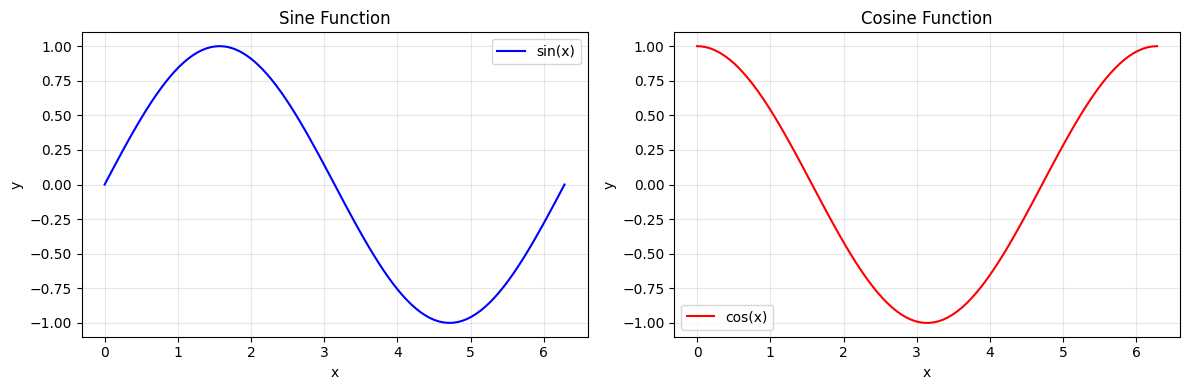
1. Subplots

Use plt.subplots() to create multiple plots in one figure:

# Create 1 row, 2 columns of subplots
fig, axes = plt.subplots(1, 2, figsize=(12, 4))

x = np.linspace(0, 2*np.pi, 100)

# First subplot
axes[0].plot(x, np.sin(x), 'b-', label='sin(x)')
axes[0].set_xlabel('x')
axes[0].set_ylabel('y')
axes[0].set_title('Sine Function')
axes[0].legend()
axes[0].grid(True, alpha=0.3)

# Second subplot
axes[1].plot(x, np.cos(x), 'r-', label='cos(x)')
axes[1].set_xlabel('x')
axes[1].set_ylabel('y')
axes[1].set_title('Cosine Function')
axes[1].legend()
axes[1].grid(True, alpha=0.3)

plt.tight_layout()  # Prevent overlap
plt.show()

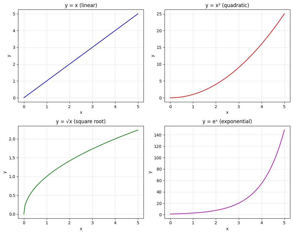
# 2x2 grid of subplots
fig, axes = plt.subplots(2, 2, figsize=(10, 8))

x = np.linspace(0, 5, 100)

# Access with [row, col]
axes[0, 0].plot(x, x, 'b-')
axes[0, 0].set_title('y = x (linear)')

axes[0, 1].plot(x, x**2, 'r-')
axes[0, 1].set_title('y = x² (quadratic)')

axes[1, 0].plot(x, np.sqrt(x), 'g-')
axes[1, 0].set_title('y = √x (square root)')

axes[1, 1].plot(x, np.exp(x), 'm-')
axes[1, 1].set_title('y = eˣ (exponential)')

# Add labels to all
for ax in axes.flat:
    ax.set_xlabel('x')
    ax.set_ylabel('y')
    ax.grid(True, alpha=0.3)

plt.tight_layout()
plt.show()

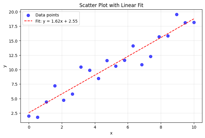
2. Different Plot Types

# Scatter plot - good for experimental data
np.random.seed(42)
x = np.linspace(0, 10, 20)
y = 2 * x + 1 + np.random.randn(20) * 2  # Linear with noise

plt.figure(figsize=(8, 5))
plt.scatter(x, y, c='blue', s=50, alpha=0.7, label='Data points')

# Add a fit line
coeffs = np.polyfit(x, y, 1)  # Linear fit
fit_line = np.poly1d(coeffs)
plt.plot(x, fit_line(x), 'r--', label=f'Fit: y = {coeffs[0]:.2f}x + {coeffs[1]:.2f}')

plt.xlabel('x')
plt.ylabel('y')
plt.title('Scatter Plot with Linear Fit')
plt.legend()
plt.grid(True, alpha=0.3)
plt.show()

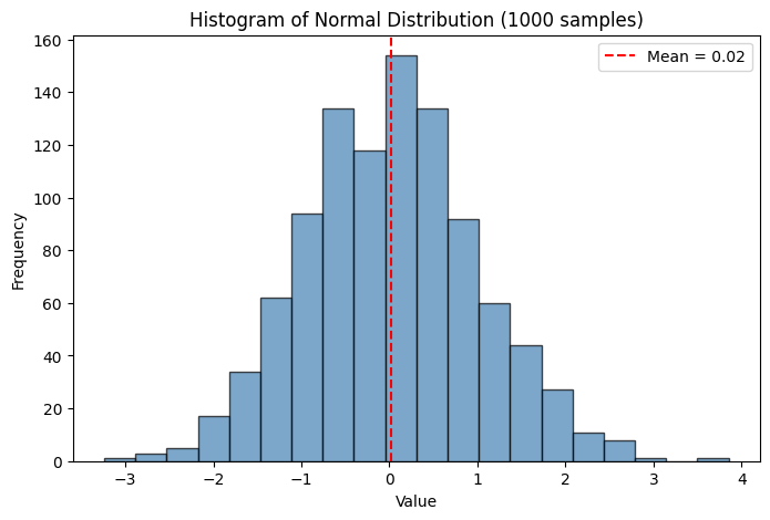
# Histogram - distribution of data
np.random.seed(42)
data = np.random.randn(1000)  # 1000 samples from normal distribution

plt.figure(figsize=(8, 5))
plt.hist(data, bins=20, color='steelblue', edgecolor='black', alpha=0.7)
plt.xlabel('Value')
plt.ylabel('Frequency')
plt.title('Histogram of Normal Distribution (1000 samples)')

# Add mean line
plt.axvline(np.mean(data), color='red', linestyle='--',
            label=f'Mean = {np.mean(data):.2f}')
plt.legend()
plt.show()

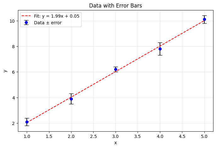
# Error bars - essential for experimental physics!
x = np.array([1, 2, 3, 4, 5])
y = np.array([2.1, 3.9, 6.2, 7.8, 10.1])
yerr = np.array([0.3, 0.4, 0.2, 0.5, 0.3])  # Uncertainties

plt.figure(figsize=(8, 5))
plt.errorbar(x, y, yerr=yerr, fmt='o', capsize=5,
             color='blue', ecolor='black', label='Data ± error')

# Fit line
coeffs = np.polyfit(x, y, 1)
plt.plot(x, np.poly1d(coeffs)(x), 'r--', label=f'Fit: y = {coeffs[0]:.2f}x + {coeffs[1]:.2f}')

plt.xlabel('x')
plt.ylabel('y')
plt.title('Data with Error Bars')
plt.legend()
plt.grid(True, alpha=0.3)
plt.show()

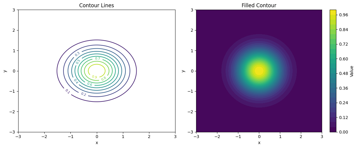
# Contour plot - for 2D data (like potential fields)
x = np.linspace(-3, 3, 100)
y = np.linspace(-3, 3, 100)
X, Y = np.meshgrid(x, y)  # Create 2D grid

# 2D Gaussian
Z = np.exp(-(X**2 + Y**2))

fig, axes = plt.subplots(1, 2, figsize=(12, 5))

# Contour lines
cs1 = axes[0].contour(X, Y, Z, levels=10, cmap='viridis')
axes[0].clabel(cs1, inline=True, fontsize=8)
axes[0].set_title('Contour Lines')
axes[0].set_xlabel('x')
axes[0].set_ylabel('y')

# Filled contour (heatmap)
cs2 = axes[1].contourf(X, Y, Z, levels=30, cmap='viridis')
plt.colorbar(cs2, ax=axes[1], label='Value')
axes[1].set_title('Filled Contour')
axes[1].set_xlabel('x')
axes[1].set_ylabel('y')

plt.tight_layout()
plt.show()

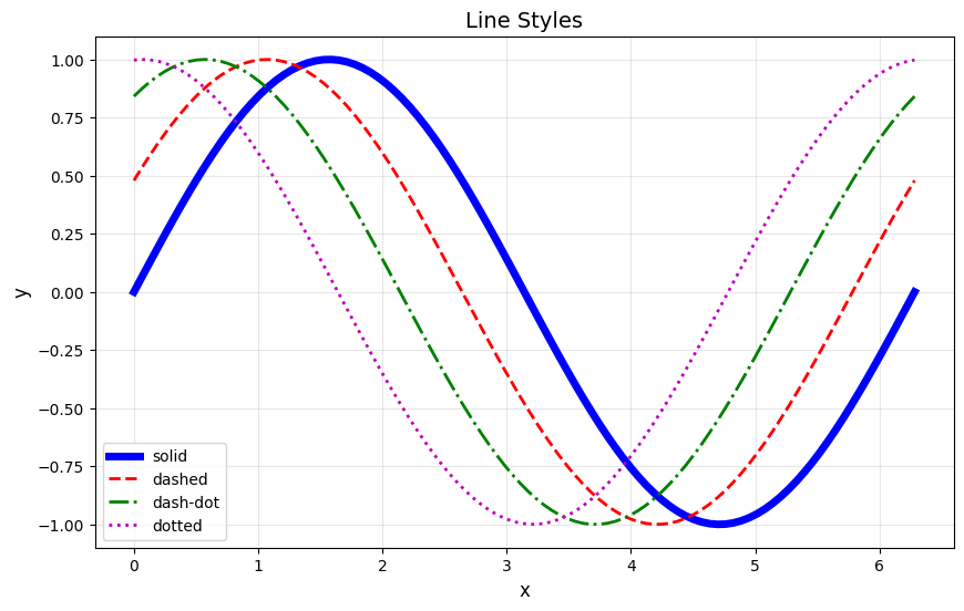
3. Customization

Make your plots publication-ready:

# Line styles and colors
x = np.linspace(0, 2*np.pi, 100)

plt.figure(figsize=(10, 6))

# Different line styles
plt.plot(x, np.sin(x), 'b-', linewidth=5, label='solid')
plt.plot(x, np.sin(x + 0.5), 'r--', linewidth=2, label='dashed')
plt.plot(x, np.sin(x + 1.0), 'g-.', linewidth=2, label='dash-dot')
plt.plot(x, np.sin(x + 1.5), 'm:', linewidth=2, label='dotted')

plt.xlabel('x', fontsize=12)
plt.ylabel('y', fontsize=12)
plt.title('Line Styles', fontsize=14)
plt.legend(fontsize=10)
plt.grid(True, alpha=0.3)
plt.show()

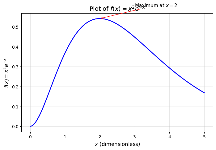
# LaTeX in labels - for proper mathematical notation
x = np.linspace(0, 5, 100)
y = x**2 * np.exp(-x)

plt.figure(figsize=(8, 5))
plt.plot(x, y, 'b-', linewidth=2)

# Use LaTeX notation with r'...' (raw string) and $...$
plt.xlabel(r'$x$ (dimensionless)', fontsize=12)
plt.ylabel(r'$f(x) = x^2 e^{-x}$', fontsize=12)
plt.title(r'Plot of $f(x) = x^2 e^{-x}$', fontsize=14)

# Add annotation with LaTeX
plt.annotate(r'Maximum at $x = 2$',
             xy=(2, 4*np.exp(-2)),
             xytext=(3, 0.6),
             fontsize=11,
             arrowprops=dict(arrowstyle='->', color='red'))

plt.grid(True, alpha=0.3)
plt.show()

4. Saving Figures

Save your plots for papers, presentations, and reports:

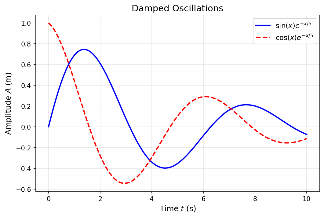
# Create a publication-quality figure
x = np.linspace(0, 10, 100)
y1 = np.sin(x) * np.exp(-x/5)
y2 = np.cos(x) * np.exp(-x/5)

fig, ax = plt.subplots(figsize=(8, 5), dpi=150)  # High DPI for quality

ax.plot(x, y1, 'b-', linewidth=2, label=r'$\sin(x) e^{-x/5}$')
ax.plot(x, y2, 'r--', linewidth=2, label=r'$\cos(x) e^{-x/5}$')

ax.set_xlabel(r'Time $t$ (s)', fontsize=12)
ax.set_ylabel(r'Amplitude $A$ (m)', fontsize=12)
ax.set_title('Damped Oscillations', fontsize=14)
ax.legend(fontsize=11)
ax.grid(True, alpha=0.3)

# Save in different formats
fig.savefig('damped_oscillation.png', dpi=300, bbox_inches='tight')
fig.savefig('damped_oscillation.pdf', bbox_inches='tight')  # Vector format

print("Saved: damped_oscillation.png and damped_oscillation.pdf")
plt.show()

Saved: damped_oscillation.png and damped_oscillation.pdf

III. Vectorization & Performance

One of the most important skills in scientific Python is writing vectorized code. This means using NumPy operations instead of Python loops.

Why vectorization matters:

• NumPy operations are implemented in C — 10-100x faster than Python loops

• Code is shorter and more readable

• Essential for large-scale simulations

1. Loop vs Vectorized: Speed Comparison

import time

# Task: compute sin(x) for 1 million points
n = 1000000
x = np.linspace(0, 2*np.pi, n)

# Method 1: Python loop (SLOW)
start = time.time()
y_loop = []
for val in x:
    y_loop.append(np.sin(val))
y_loop = np.array(y_loop)
loop_time = time.time() - start
print(f"Python loop: {loop_time:.4f} seconds")

# Method 2: Vectorized (FAST)
start = time.time()
y_vec = np.sin(x)
vec_time = time.time() - start
print(f"Vectorized:  {vec_time:.4f} seconds")

print(f"\nSpeedup: {loop_time/vec_time:.1f}x faster!")

Python loop: 1.1931 seconds
Vectorized:  0.0140 seconds

Speedup: 85.3x faster!

2. Vectorization Examples

Learn to think in arrays, not loops:

# Example 1: Compute kinetic energy for many particles
masses = np.array([1.0, 2.0, 0.5, 1.5, 3.0])      # kg
velocities = np.array([10, 5, 20, 8, 4])          # m/s

# Vectorized: all at once!
kinetic_energies = 0.5 * masses * velocities**2

print("Masses (kg):    ", masses)
print("Velocities (m/s):", velocities)
print("KE (J):         ", kinetic_energies)
print(f"Total KE: {np.sum(kinetic_energies):.1f} J")

Masses (kg):     [1.  2.  0.5 1.5 3. ]
Velocities (m/s): [10  5 20  8  4]
KE (J):          [ 50.  25. 100.  48.  24.]
Total KE: 247.0 J

# Example 2: Distance between all pairs of points
# (This would require nested loops without vectorization)

# 5 particles in 2D
x = np.array([0, 1, 2, 3, 4])
y = np.array([0, 1, 0, 1, 0])

# n = len(x)
# for i in range(5):
#     for j in range(5):
#         dx = x[i] - x[j]
#         dy = y[i] - y[j]
#         distances = np.sqrt(dx**2 + dy**2)

# Compute pairwise distances using broadcasting
# We need to reshape to enable broadcasting
dx = x[:, np.newaxis] - x[np.newaxis, :]  # 5x5 matrix of x-differences
dy = y[:, np.newaxis] - y[np.newaxis, :]  # 5x5 matrix of y-differences
distances = np.sqrt(dx**2 + dy**2)

print("Particle positions:")
for i in range(len(x)):
    print(f"  Particle {i}: ({x[i]}, {y[i]})")

print("\nDistance matrix:")
print(np.round(distances, 2))

Particle positions:
  Particle 0: (0, 0)
  Particle 1: (1, 1)
  Particle 2: (2, 0)
  Particle 3: (3, 1)
  Particle 4: (4, 0)

Distance matrix:
[[0.   1.41 2.   3.16 4.  ]
 [1.41 0.   1.41 2.   3.16]
 [2.   1.41 0.   1.41 2.  ]
 [3.16 2.   1.41 0.   1.41]
 [4.   3.16 2.   1.41 0.  ]]

3. Common Vectorization Patterns

Loop Version	Vectorized Version
for x in arr: result.append(f(x))	result = f(arr)
for i in range(n): total += arr[i]	total = np.sum(arr)
for i in range(n): if arr[i] > 0: ...	arr[arr > 0]
for i in range(n): arr[i] = arr[i] * 2	arr = arr * 2

IV. Functions as Arguments

In Python, functions are first-class objects — they can be passed as arguments to other functions. This is essential for numerical methods!

For example, a numerical integrator needs to know which function to integrate. You pass the function itself as an argument.

1. Passing Functions to Functions

# A function that takes another function as an argument
def apply_twice(func, x):
    """Apply a function twice: func(func(x))"""
    return func(func(x))

def square(x):
    return x ** 2

def add_one(x):
    return x + 1

# Pass different functions
print(f"square applied twice to 2: {apply_twice(square, 2)}")   # (2²)² = 16
print(f"add_one applied twice to 5: {apply_twice(add_one, 5)}") # 5+1+1 = 7
print(f"np.sin applied twice to π/2: {apply_twice(np.sin, np.pi/2):.4f}")  # sin(sin(π/2))

square applied twice to 2: 16
add_one applied twice to 5: 7
np.sin applied twice to π/2: 0.8415

2. Preview: Numerical Derivative

This is exactly how we’ll implement numerical differentiation in the next lecture:

\[f'(x) \approx \frac{f(x+h) - f(x)}{h}\]

def numerical_derivative(f, x, h=1e-5):
    """
    Compute the derivative of f at x using finite difference.

    Parameters:
        f: function to differentiate
        x: point at which to compute derivative
        h: step size (smaller = more accurate, but can cause numerical issues)

    Returns:
        Approximate derivative f'(x)
    """
    return (f(x + h) - f(x)) / h

# Test with known derivatives
print("Testing numerical derivative:")
print(f"d/dx[sin(x)] at x=0: {numerical_derivative(np.sin, 0):.6f} (exact: {np.cos(0)})")
print(f"d/dx[x²] at x=3: {numerical_derivative(lambda x: x**2, 3):.6f} (exact: 6)")
print(f"d/dx[eˣ] at x=1: {numerical_derivative(np.exp, 1):.6f} (exact: {np.exp(1):.6f})")

Testing numerical derivative:
d/dx[sin(x)] at x=0: 1.000000 (exact: 1.0)
d/dx[x²] at x=3: 6.000010 (exact: 6)
d/dx[eˣ] at x=1: 2.718295 (exact: 2.718282)

3. Lambda Functions

Lambda functions are small, anonymous functions defined in one line. They’re convenient when you need a simple function just once:

# Lambda syntax: lambda arguments: expression

# Instead of:
def square(x):
    return x ** 2

# You can write:
square_lambda = lambda x: x ** 2

print(f"square(5) = {square(5)}")
print(f"square_lambda(5) = {square_lambda(5)}")

# More examples
add = lambda x, y: x + y
print(f"add(3, 4) = {add(3, 4)}")

def addd(x,y):
    return x+y

# Often used inline:
print(f"Derivative of x³ at x=2: {numerical_derivative(lambda x: x**3, 2)}")

# Physics example: Compute derivatives of various potentials

# Harmonic oscillator: V(x) = 0.5 * k * x²
# Gravitational: V(r) = -G*M*m / r
# Lennard-Jones: V(r) = 4ε[(σ/r)¹² - (σ/r)⁶]

k = 1.0  # spring constant
harmonic = lambda x: 0.5 * k * x**2

# Force = -dV/dx
x = 2.0
force = -numerical_derivative(harmonic, x)
print(f"Harmonic potential at x={x}: V = {harmonic(x)}")
print(f"Force at x={x}: F = {force:.4f} (exact: {-k*x})")

Harmonic potential at x=2.0: V = 2.0
Force at x=2.0: F = -2.0000 (exact: -2.0)

V. Physics Applications

Let’s put everything together with complete physics examples!

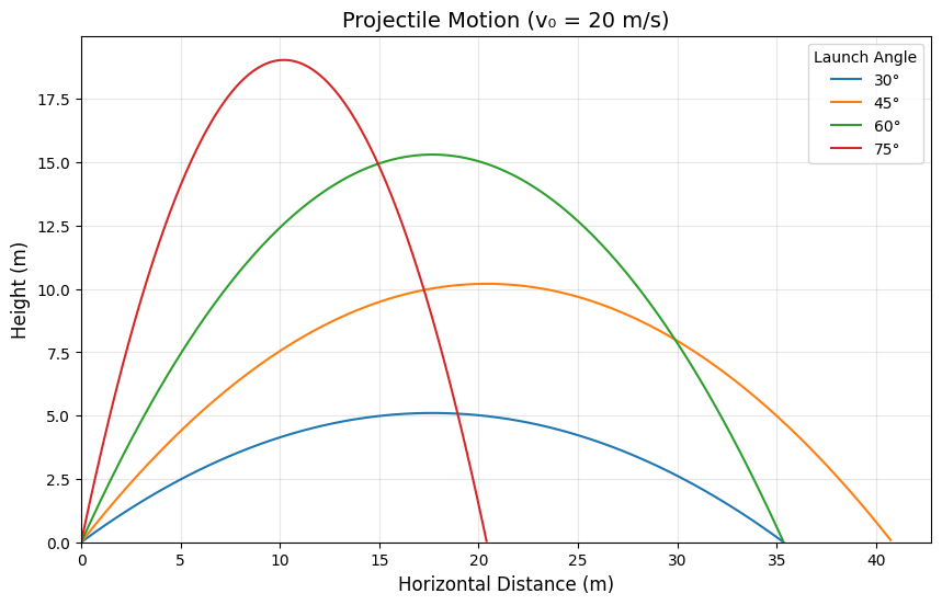
1. Projectile Motion

Simulate and visualize projectile motion with different launch angles:

def projectile_motion(v0, theta_deg, g=9.8, dt=0.01):
    """
    Simulate projectile motion.

    Parameters:
        v0: initial velocity (m/s)
        theta_deg: launch angle (degrees)
        g: gravitational acceleration (m/s²)
        dt: time step (s)

    Returns:
        t, x, y: time array, x positions, y positions
    """
    theta = np.radians(theta_deg)
    v0x = v0 * np.cos(theta)
    v0y = v0 * np.sin(theta)

    # Time of flight (when y = 0 again)
    t_flight = 2 * v0y / g

    # Create time array
    t = np.arange(0, t_flight, dt)

    # Compute trajectory (vectorized!)
    x = v0x * t
    y = v0y * t - 0.5 * g * t**2

    return t, x, y

# Compare different launch angles
v0 = 20  # m/s
angles = [30, 45, 60, 75]

plt.figure(figsize=(10, 6))

for angle in angles:
    t, x, y = projectile_motion(v0, angle)
    plt.plot(x, y, label=f'{angle}°')

plt.xlabel('Horizontal Distance (m)', fontsize=12)
plt.ylabel('Height (m)', fontsize=12)
plt.title(f'Projectile Motion (v₀ = {v0} m/s)', fontsize=14)
plt.legend(title='Launch Angle')
plt.grid(True, alpha=0.3)
plt.xlim(0, None)
plt.ylim(0, None)
plt.show()

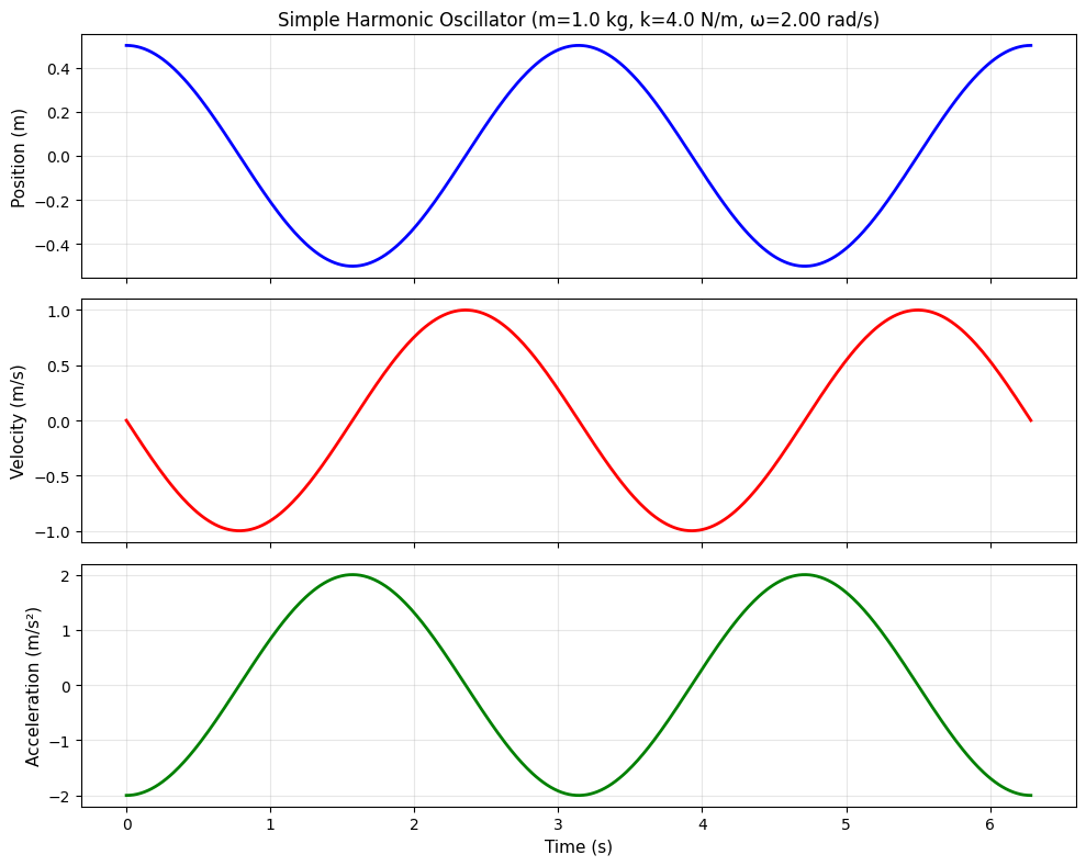
2. Simple Harmonic Oscillator

A preview of differential equations — the motion of a mass on a spring:

\[x(t) = A \cos(\omega t + \phi)\]

where \(\omega = \sqrt{k/m}\)

def harmonic_oscillator(t, A, omega, phi=0):
    """
    Simple harmonic oscillator solution.

    Parameters:
        t: time array
        A: amplitude
        omega: angular frequency (rad/s)
        phi: phase (rad)

    Returns:
        x: position, v: velocity, a: acceleration
    """
    x = A * np.cos(omega * t + phi)
    v = -A * omega * np.sin(omega * t + phi)
    a = -A * omega**2 * np.cos(omega * t + phi)
    return x, v, a

# Parameters
m = 1.0    # mass (kg)
k = 4.0    # spring constant (N/m)
A = 0.5    # amplitude (m)
omega = np.sqrt(k / m)  # angular frequency

t = np.linspace(0, 4*np.pi/omega, 500)  # 2 complete periods
x, v, a = harmonic_oscillator(t, A, omega)

# Visualization
fig, axes = plt.subplots(3, 1, figsize=(10, 8), sharex=True)

axes[0].plot(t, x, 'b-', linewidth=2)
axes[0].set_ylabel('Position (m)', fontsize=11)
axes[0].set_title(f'Simple Harmonic Oscillator (m={m} kg, k={k} N/m, ω={omega:.2f} rad/s)', fontsize=12)
axes[0].grid(True, alpha=0.3)

axes[1].plot(t, v, 'r-', linewidth=2)
axes[1].set_ylabel('Velocity (m/s)', fontsize=11)
axes[1].grid(True, alpha=0.3)

axes[2].plot(t, a, 'g-', linewidth=2)
axes[2].set_ylabel('Acceleration (m/s²)', fontsize=11)
axes[2].set_xlabel('Time (s)', fontsize=11)
axes[2].grid(True, alpha=0.3)

plt.tight_layout()
plt.show()

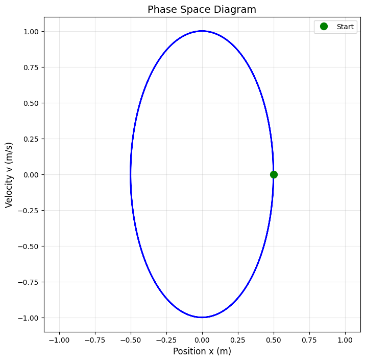
# Phase space diagram (position vs velocity)
plt.figure(figsize=(8, 8))
plt.plot(x, v, 'b-', linewidth=2)
plt.xlabel('Position x (m)', fontsize=12)
plt.ylabel('Velocity v (m/s)', fontsize=12)
plt.title('Phase Space Diagram', fontsize=14)
plt.grid(True, alpha=0.3)
plt.axis('equal')

# Mark the starting point
plt.plot(x[0], v[0], 'go', markersize=10, label='Start')
plt.legend()
plt.show()

# Verify energy conservation
KE = 0.5 * m * v**2           # Kinetic energy
PE = 0.5 * k * x**2           # Potential energy
total_energy = KE + PE

fig, axes = plt.subplots(2, 1, figsize=(10, 6), sharex=True)

axes[0].plot(t, KE, 'r-', label='Kinetic Energy', linewidth=2)
axes[0].plot(t, PE, 'b-', label='Potential Energy', linewidth=2)
axes[0].set_ylabel('Energy (J)', fontsize=11)
axes[0].legend()
axes[0].grid(True, alpha=0.3)
axes[0].set_title('Energy in Simple Harmonic Oscillator', fontsize=12)

axes[1].plot(t, total_energy, 'k-', linewidth=2)
axes[1].set_ylabel('Total Energy (J)', fontsize=11)
axes[1].set_xlabel('Time (s)', fontsize=11)
axes[1].set_ylim([0, 1.1*max(total_energy)])
axes[1].grid(True, alpha=0.3)

plt.tight_layout()
plt.show()

print(f"Total energy varies by: {(max(total_energy)-min(total_energy))/np.mean(total_energy)*100:.2e}%")
print("(Should be constant - variation is due to numerical precision)")

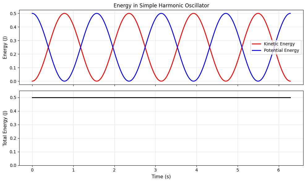
Total energy varies by: 4.44e-14%
(Should be constant - variation is due to numerical precision)

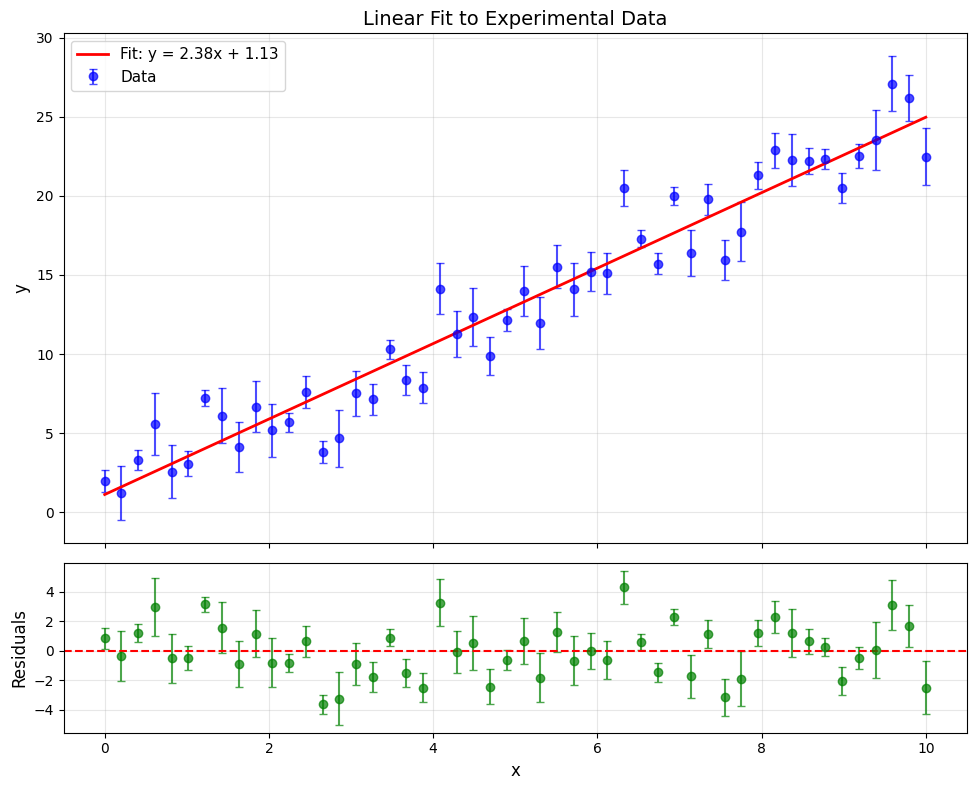
3. Experimental Data Analysis

A complete workflow: load data, analyze, visualize, save results.

# Generate synthetic "experimental" data
np.random.seed(42)
n_points = 50

# True relationship: y = 2.5x + 1.0 with noise
x_data = np.linspace(0, 10, n_points)
y_true = 2.5 * x_data + 1.0
y_noise = np.random.normal(0, 2, n_points)
y_data = y_true + y_noise
y_errors = np.random.uniform(0.5, 2.0, n_points)  # Uncertainties

# Save to file
np.savetxt('experiment_data.csv',
           np.column_stack([x_data, y_data, y_errors]),
           delimiter=',',
           header='x,y,y_error',
           comments='')
print("Saved: experiment_data.csv")

Saved: experiment_data.csv

# Load and analyze the data
data = np.loadtxt('experiment_data.csv', delimiter=',', skiprows=1)
x = data[:, 0]
y = data[:, 1]
yerr = data[:, 2]

# Fit a line
coeffs = np.polyfit(x, y, 1)
slope, intercept = coeffs
y_fit = np.poly1d(coeffs)(x)

# Statistics
residuals = y - y_fit
chi_squared = np.sum((residuals / yerr)**2)
dof = len(y) - 2  # degrees of freedom

print("=== Analysis Results ===")
print(f"Slope: {slope:.3f}")
print(f"Intercept: {intercept:.3f}")
print(f"χ²/dof: {chi_squared/dof:.2f}")

# Publication-quality plot
fig, axes = plt.subplots(2, 1, figsize=(10, 8),
                         gridspec_kw={'height_ratios': [3, 1]}, sharex=True)

# Main plot
axes[0].errorbar(x, y, yerr=yerr, fmt='o', capsize=3,
                 color='blue', alpha=0.7, label='Data')
axes[0].plot(x, y_fit, 'r-', linewidth=2,
             label=f'Fit: y = {slope:.2f}x + {intercept:.2f}')
axes[0].set_ylabel('y', fontsize=12)
axes[0].set_title('Linear Fit to Experimental Data', fontsize=14)
axes[0].legend(fontsize=11)
axes[0].grid(True, alpha=0.3)

# Residuals
axes[1].errorbar(x, residuals, yerr=yerr, fmt='o', capsize=3, color='green', alpha=0.7)
axes[1].axhline(y=0, color='r', linestyle='--')
axes[1].set_xlabel('x', fontsize=12)
axes[1].set_ylabel('Residuals', fontsize=12)
axes[1].grid(True, alpha=0.3)

plt.tight_layout()
plt.savefig('analysis_result.png', dpi=300, bbox_inches='tight')
print("\nSaved: analysis_result.png")
plt.show()

=== Analysis Results ===
Slope: 2.384
Intercept: 1.129
χ²/dof: 3.71

Saved: analysis_result.png

VI. Summary

What We Learned Today

NumPy Arrays

• Creating arrays: np.array(), np.zeros(), np.linspace(), np.arange()

• Array operations: element-wise math, broadcasting, universal functions

• Indexing: slicing, boolean indexing (filtering)

• Methods: sum(), mean(), std(), min(), max(), diff(), cumsum()

Advanced Matplotlib

• Subplots: plt.subplots(rows, cols)

• Plot types: scatter(), hist(), errorbar(), contour()

• Customization: labels, LaTeX, styles

• Saving: plt.savefig()

Vectorization

• NumPy operations are 10-100x faster than Python loops

• Think in arrays, not loops

• Use boolean indexing for filtering

Functions as Arguments

• Functions can be passed to other functions

• Lambda functions for quick, anonymous functions

• Essential for numerical methods (integration, differentiation, root finding)