The Fourier Transform

Any signal — no matter how complex — can be decomposed into a sum of simple sine and cosine waves.

Why Fourier Analysis?

Time Domain	Frequency Domain
What happens at each moment	What frequencies are present
Natural for measurement	Natural for understanding
Convolution is hard	Convolution becomes multiplication
Differential equations are hard	Become algebraic equations

Note: We focus on understanding the mathematics and implementation of the DFT. The Fast Fourier Transform (FFT) algorithm will be covered in the next lecture.

import numpy as np
import matplotlib.pyplot as plt

# For nicer plots (projector-friendly)
plt.rcParams['figure.figsize'] = [6, 4]
plt.rcParams['font.size'] = 9

I. The Big Idea: Building Signals from Sines

Joseph Fourier (1807) showed that any periodic function can be written as a sum of sines and cosines:

\[f(t) = \frac{a_0}{2} + \sum_{n=1}^{\infty} \left[ a_n \cos\left(\frac{2\pi n t}{T}\right) + b_n \sin\left(\frac{2\pi n t}{T}\right) \right]\]

where \(T\) is the period. This is the Fourier Series.

Let’s see this in action — building a square wave from sines.

# Build a square wave from sine waves!
t = np.linspace(0, 2, 1000)  # 2 periods

# Square wave Fourier series: f(t) = (4/pi) * sum[ sin(n*pi*t) / n ] for odd n
plt.figure(figsize=(6, 8))

n_terms_list = [1, 3, 9, 5000]
for idx, N in enumerate(n_terms_list):
    plt.subplot(4, 1, idx + 1)

    # Build the partial sum
    f = np.zeros_like(t)
    for n in range(1, N + 1, 2):  # odd n only
        f += (4 / np.pi) * np.sin(2 * np.pi * n * t / 2) / n

    plt.plot(t, f, 'b-', linewidth=2, label=f'{(N+1)//2} terms')

    # True square wave for reference
    square = np.sign(np.sin(2 * np.pi * t / 2))
    plt.plot(t, square, 'r--', linewidth=1, alpha=0.5, label='True square wave')

    plt.ylim(-1.5, 1.5)
    plt.ylabel('f(t)')
    plt.legend(loc='upper right', fontsize=8)
    plt.grid(True, alpha=0.3)
    if idx < 3:
        plt.tick_params(labelbottom=False)

plt.xlabel('t')
plt.suptitle('Building a Square Wave from Sine Waves', y=1.01)
plt.tight_layout()
plt.show()

print('More terms → better approximation!')
print('Notice the overshoot at the edges — this is the Gibbs phenomenon.')

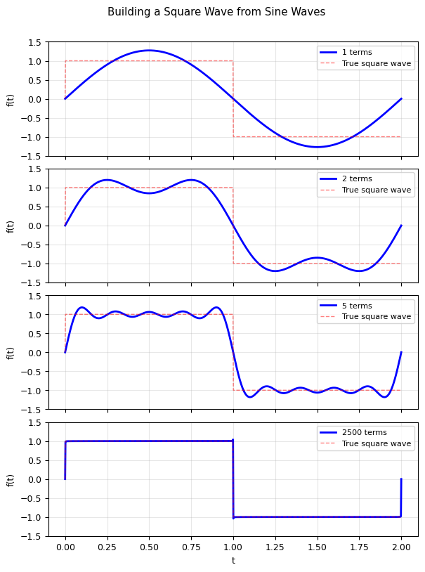
More terms → better approximation!
Notice the overshoot at the edges — this is the Gibbs phenomenon.

II. Fourier Series Coefficients

For a periodic function \(f(t)\) with period \(T\), the Fourier coefficients are:

Cosine coefficients

\[a_n = \frac{2}{T} \int_0^T f(t) \cos\left(\frac{2\pi n t}{T}\right) dt\]

Sine coefficients

\[b_n = \frac{2}{T} \int_0^T f(t) \sin\left(\frac{2\pi n t}{T}\right) dt\]

DC component (average value)

\[a_0 = \frac{2}{T} \int_0^T f(t) \, dt\]

Why does this work?

Orthogonality! Sine and cosine functions are orthogonal over one period:

\[\begin{split}\int_0^T \sin\left(\frac{2\pi m t}{T}\right) \sin\left(\frac{2\pi n t}{T}\right) dt = \begin{cases} T/2 & \text{if } m = n \\ 0 & \text{if } m \neq n \end{cases}\end{split}\]

This is just like dot products of orthogonal vectors — we “project” the signal onto each basis function.

# Hand-implement Fourier coefficient computation
# using numerical integration (trapezoidal rule from Lecture 04!)

def fourier_coefficients(f_values, t, T, N_max):
    """
    Compute Fourier series coefficients numerically.

    Parameters:
        f_values: array of function values over one period
        t: array of time points over one period
        T: period of the function
        N_max: number of harmonics to compute

    Returns:
        a: array of cosine coefficients [a0, a1, a2, ...]
        b: array of sine coefficients [0, b1, b2, ...]
    """
    a = np.zeros(N_max + 1)
    b = np.zeros(N_max + 1)

    for n in range(N_max + 1):
        # Compute a_n using trapezoidal integration np.trapz()
        # using the formula: a_n = (2/T) * ∫ f(t) * cos(2πnt/T) dt
        integrand_a = f_values * np.cos(2 * np.pi * n * t / T)
        a[n] = (2/T) * np.trapz(integrand_a, t)

        # Compute b_n using trapezoidal integration np.trapz()
        # using the formula: b_n = (2/T) * ∫ f(t) * sin(2πnt/T) dt
        integrand_b = f_values * np.sin(2 * np.pi * n * t / T)
        b[n] = (2/T) * np.trapz(integrand_b, t)

    return a, b

# Test: compute coefficients of a square wave
T = 2.0  # period
t_period = np.linspace(0, T, 1000, endpoint=False)
square_wave = np.sign(np.sin(2 * np.pi * t_period / T))

N_max = 10
a_coeffs, b_coeffs = fourier_coefficients(square_wave, t_period, T, N_max)

print('Fourier coefficients of a square wave:')
print('=' * 45)
print(f'{"n":>3s}  {"a_n":>10s}  {"b_n":>10s}  {"expected b_n":>12s}')
print('-' * 45)
for n in range(N_max + 1):
    expected = 4 / (np.pi * n) if (n > 0 and n % 2 == 1) else 0
    print(f'{n:3d}  {a_coeffs[n]:10.4f}  {b_coeffs[n]:10.4f}  {expected:12.4f}')

print('\nAll a_n ≈ 0 (square wave is odd → no cosine terms)')
print('b_n = 4/(nπ) for odd n, 0 for even n')

Fourier coefficients of a square wave:
=============================================
  n         a_n         b_n  expected b_n
---------------------------------------------
  0      0.0030      0.0000        0.0000
  1     -0.0010      1.2732        1.2732
  2      0.0030     -0.0000        0.0000
  3     -0.0010      0.4244        0.4244
  4      0.0030     -0.0000        0.0000
  5     -0.0010      0.2546        0.2546
  6      0.0030     -0.0000        0.0000
  7     -0.0010      0.1818        0.1819
  8      0.0030     -0.0001        0.0000
  9     -0.0010      0.1414        0.1415
 10      0.0030     -0.0001        0.0000

All a_n ≈ 0 (square wave is odd → no cosine terms)
b_n = 4/(nπ) for odd n, 0 for even n

/tmp/ipython-input-1056247226.py:25: DeprecationWarning: `trapz` is deprecated. Use `trapezoid` instead, or one of the numerical integration functions in `scipy.integrate`.
  a[n] = (2/T) * np.trapz(integrand_a, t)
/tmp/ipython-input-1056247226.py:30: DeprecationWarning: `trapz` is deprecated. Use `trapezoid` instead, or one of the numerical integration functions in `scipy.integrate`.
  b[n] = (2/T) * np.trapz(integrand_b, t)

# Visualize the Fourier spectrum
plt.figure(figsize=(6, 8))

# Top: the signal
plt.subplot(2, 1, 1)
plt.plot(t_period, square_wave, 'b-', linewidth=2)
plt.xlabel('t')
plt.ylabel('f(t)')
plt.title('Square Wave (One Period)')
plt.grid(True, alpha=0.3)

# Bottom: the frequency spectrum
plt.subplot(2, 1, 2)
n_vals = np.arange(N_max + 1)
plt.stem(n_vals, np.abs(b_coeffs), linefmt='r-', markerfmt='ro', basefmt='k-',
         label='|b_n| (sine)')
plt.stem(n_vals, np.abs(a_coeffs), linefmt='b-', markerfmt='bs', basefmt='k-',
         label='|a_n| (cosine)')
plt.xlabel('Harmonic number n')
plt.ylabel('Coefficient magnitude')
plt.title('Fourier Spectrum')
plt.legend()
plt.grid(True, alpha=0.3)

plt.tight_layout()
plt.show()

print('The spectrum tells us WHICH frequencies are present and HOW MUCH of each.')

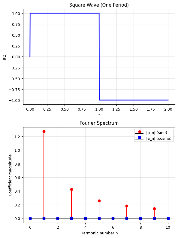
The spectrum tells us WHICH frequencies are present and HOW MUCH of each.

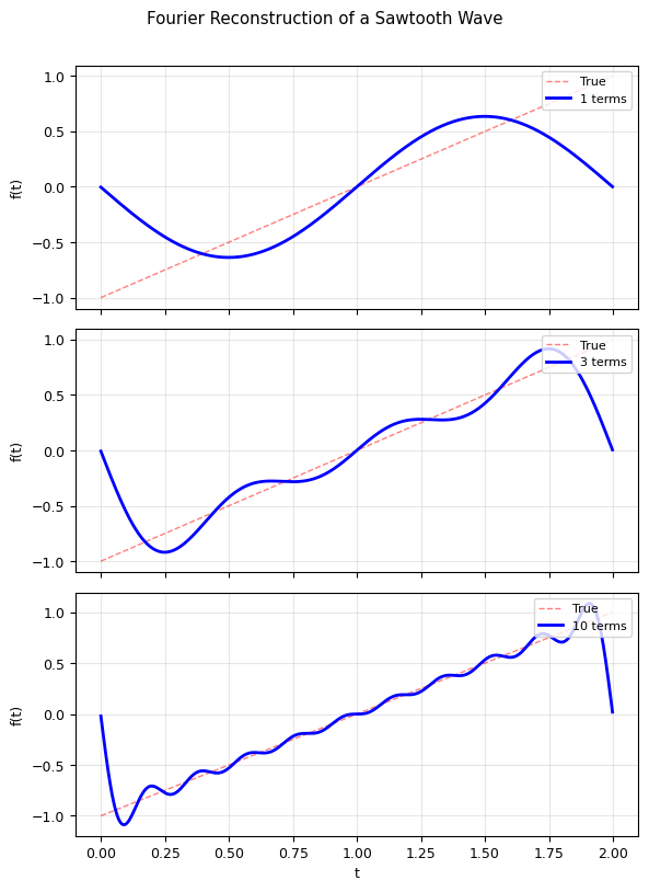
Example: Sawtooth Wave

# Sawtooth wave: f(t) = t/T on [0, T), periodic
sawtooth = 2 * (t_period / T) - 1  # Range [-1, 1]

a_saw, b_saw = fourier_coefficients(sawtooth, t_period, T, N_max)

# Reconstruct with increasing number of terms
plt.figure(figsize=(6, 8))

for idx, N in enumerate([1, 3, 10]):
    plt.subplot(3, 1, idx + 1)

    # Reconstruct
    f_approx = a_saw[0] / 2
    for n in range(1, N + 1):
        f_approx += a_saw[n] * np.cos(2 * np.pi * n * t_period / T)
        f_approx += b_saw[n] * np.sin(2 * np.pi * n * t_period / T)

    plt.plot(t_period, sawtooth, 'r--', linewidth=1, alpha=0.5, label='True')
    plt.plot(t_period, f_approx, 'b-', linewidth=2, label=f'{N} terms')
    plt.ylabel('f(t)')
    plt.legend(loc='upper right', fontsize=8)
    plt.grid(True, alpha=0.3)
    if idx < 2:
        plt.tick_params(labelbottom=False)

plt.xlabel('t')
plt.suptitle('Fourier Reconstruction of a Sawtooth Wave', y=1.01)
plt.tight_layout()
plt.show()

/tmp/ipython-input-1056247226.py:25: DeprecationWarning: `trapz` is deprecated. Use `trapezoid` instead, or one of the numerical integration functions in `scipy.integrate`.
  a[n] = (2/T) * np.trapz(integrand_a, t)
/tmp/ipython-input-1056247226.py:30: DeprecationWarning: `trapz` is deprecated. Use `trapezoid` instead, or one of the numerical integration functions in `scipy.integrate`.
  b[n] = (2/T) * np.trapz(integrand_b, t)

III. Complex Fourier Series

Using Euler’s formula \(e^{i\theta} = \cos\theta + i\sin\theta\), we can write the Fourier series more compactly:

\[f(t) = \sum_{n=-\infty}^{\infty} c_n \, e^{i 2\pi n t / T}\]

where the complex coefficients are:

\[c_n = \frac{1}{T} \int_0^T f(t) \, e^{-i 2\pi n t / T} \, dt\]

Relationship to \(a_n\) and \(b_n\)

\[c_n = \frac{1}{2}(a_n - i \, b_n) \quad \text{for } n > 0\]

\[c_0 = \frac{a_0}{2} \quad \text{(DC component)}\]

The amplitude spectrum is \(|c_n|\) and the power spectrum is \(|c_n|^2\).

Why complex?

• More compact notation

• Easier to manipulate mathematically

• Natural for the DFT and FFT

• Negative frequencies have physical meaning (rotation direction)

# Hand-implement complex Fourier coefficients
def complex_fourier_coefficients(f_values, t, T, N_max):
    """
    Compute complex Fourier coefficients c_n.

    Parameters:
        f_values: function values over one period
        t: time array over one period
        T: period
        N_max: compute c_{-N_max} to c_{N_max}

    Returns:
        n_vals: array of n values from -N_max to N_max
        c_n: complex coefficients
    """
    n_vals = np.arange(-N_max, N_max + 1)
    c_n = np.zeros(len(n_vals), dtype=complex)

    for i, n in enumerate(n_vals):
        # c_n = (1/T) * integral of f(t) * exp(-i*2*pi*n*t/T) dt
        integrand = f_values * np.exp(-1j * 2 * np.pi * n * t / T)
        c_n[i] = (1 / T) * np.trapz(integrand, t)

    return n_vals, c_n

# Compute for the square wave
n_vals, c_n = complex_fourier_coefficients(square_wave, t_period, T, N_max)

# Plot amplitude spectrum
plt.figure(figsize=(6, 5))
plt.stem(n_vals, np.abs(c_n), linefmt='b-', markerfmt='bo', basefmt='k-')
plt.xlabel('Harmonic number n')
plt.ylabel('|c_n|')
plt.title('Complex Fourier Spectrum of Square Wave')
plt.grid(True, alpha=0.3)
plt.tight_layout()
plt.show()

print('Note: the spectrum is symmetric — |c_n| = |c_{-n}| for real signals.')
print('This symmetry means negative frequencies are redundant (for real signals).')

/tmp/ipython-input-727021825.py:22: DeprecationWarning: `trapz` is deprecated. Use `trapezoid` instead, or one of the numerical integration functions in `scipy.integrate`.
  c_n[i] = (1 / T) * np.trapz(integrand, t)

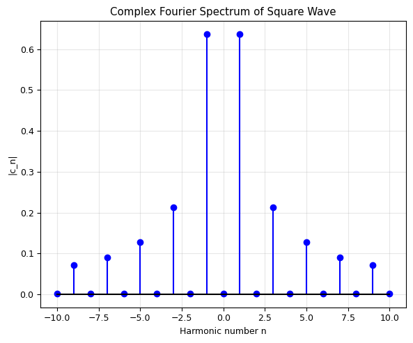
Note: the spectrum is symmetric — |c_n| = |c_{-n}| for real signals.
This symmetry means negative frequencies are redundant (for real signals).

IV. From Fourier Series to Fourier Transform

The Fourier Series works for periodic functions. What about non-periodic functions?

Key idea: Let the period \(T \to \infty\). Then:

• The discrete harmonics \(n/T\) become a continuous frequency \(f\)

• The sum becomes an integral

• The coefficients \(c_n\) become a continuous function \(\hat{f}(\nu)\)

The Fourier Transform Pair

Forward Transform (time → frequency):

\[\hat{f}(\nu) = \int_{-\infty}^{\infty} f(t) \, e^{-i 2\pi \nu t} \, dt\]

Inverse Transform (frequency → time):

\[f(t) = \int_{-\infty}^{\infty} \hat{f}(\nu) \, e^{i 2\pi \nu t} \, d\nu\]

Alternative convention (angular frequency \(\omega = 2\pi\nu\))

\[\hat{f}(\omega) = \int_{-\infty}^{\infty} f(t) \, e^{-i \omega t} \, dt \qquad f(t) = \frac{1}{2\pi}\int_{-\infty}^{\infty} \hat{f}(\omega) \, e^{i \omega t} \, d\omega\]

Warning: Different textbooks use different conventions for the \(2\pi\) factor! Always check which convention is being used.

Example: Fourier Transform of a Gaussian

A Gaussian pulse: \(f(t) = e^{-\alpha t^2}\)

Its Fourier transform is also a Gaussian:

\[\hat{f}(\nu) = \sqrt{\frac{\pi}{\alpha}} \, e^{-\pi^2 \nu^2 / \alpha}\]

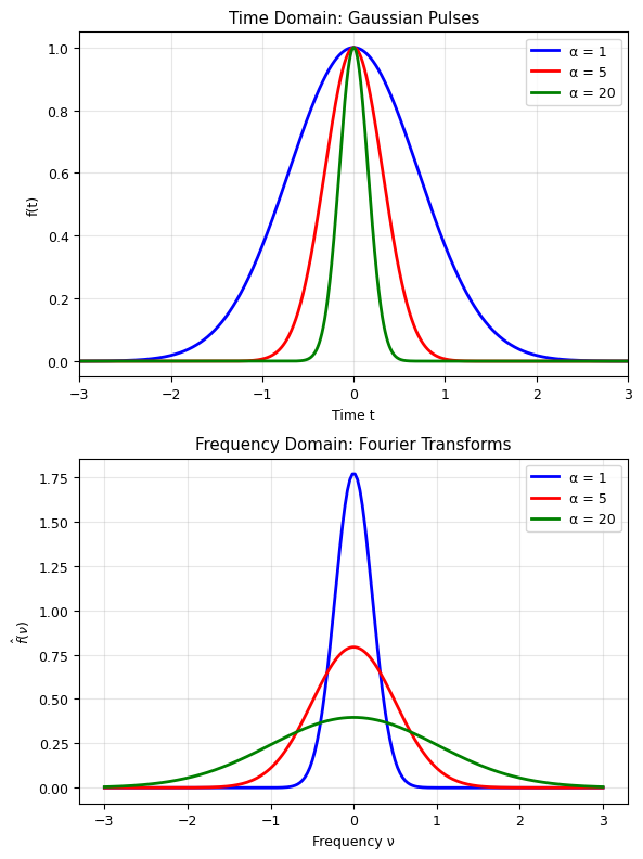
Key insight: A narrow pulse in time → a wide spectrum in frequency (and vice versa). This is the uncertainty principle!

# Fourier Transform of a Gaussian — numerical vs analytical
def numerical_fourier_transform(f_values, t, freqs):
    """
    Compute the continuous Fourier transform numerically
    using trapezoidal integration.

    Parameters:
        f_values: function values at time points t
        t: time array
        freqs: frequency array to evaluate at

    Returns:
        F: complex Fourier transform values
    """
    F = np.zeros(len(freqs), dtype=complex)
    for i, nu in enumerate(freqs):
        integrand = f_values * np.exp(-1j * 2 * np.pi * nu * t)
        F[i] = np.trapz(integrand, t)
    return F

# Gaussian pulse
alpha = 5.0
t_ft = np.linspace(-5, 5, 2000)
gaussian_pulse = np.exp(-alpha * t_ft**2)

# Numerical FT
freqs = np.linspace(-3, 3, 200)
F_numerical = numerical_fourier_transform(gaussian_pulse, t_ft, freqs)

# Analytical FT
F_analytical = np.sqrt(np.pi / alpha) * np.exp(-np.pi**2 * freqs**2 / alpha)

plt.figure(figsize=(6, 8))

plt.subplot(2, 1, 1)
plt.plot(t_ft, gaussian_pulse, 'b-', linewidth=2)
plt.xlabel('Time t')
plt.ylabel('f(t)')
plt.title(f'Gaussian Pulse: $f(t) = e^{{-{alpha}t^2}}$')
plt.grid(True, alpha=0.3)

plt.subplot(2, 1, 2)
plt.plot(freqs, np.real(F_numerical), 'b-', linewidth=2, label='Numerical FT')
plt.plot(freqs, F_analytical, 'r--', linewidth=2, label='Analytical FT')
plt.xlabel('Frequency ν')
plt.ylabel('$\\hat{f}(\\nu)$')
plt.title('Fourier Transform (also a Gaussian!)')
plt.legend()
plt.grid(True, alpha=0.3)

plt.tight_layout()
plt.show()

print(f'Max error between numerical and analytical: {np.max(np.abs(np.real(F_numerical) - F_analytical)):.6f}')
print('The Fourier transform of a Gaussian is a Gaussian!')

/tmp/ipython-input-3070628031.py:18: DeprecationWarning: `trapz` is deprecated. Use `trapezoid` instead, or one of the numerical integration functions in `scipy.integrate`.
  F[i] = np.trapz(integrand, t)

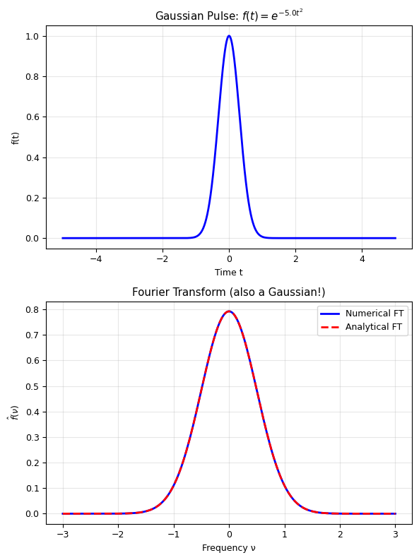
Max error between numerical and analytical: 0.000000
The Fourier transform of a Gaussian is a Gaussian!

# The Uncertainty Principle: narrow in time ↔ wide in frequency
plt.figure(figsize=(6, 8))

alphas = [1, 5, 20]
colors = ['b', 'r', 'g']

plt.subplot(2, 1, 1)
for alpha_val, c in zip(alphas, colors):
    pulse = np.exp(-alpha_val * t_ft**2)
    plt.plot(t_ft, pulse, c + '-', linewidth=2, label=f'α = {alpha_val}')
plt.xlabel('Time t')
plt.ylabel('f(t)')
plt.title('Time Domain: Gaussian Pulses')
plt.legend()
plt.grid(True, alpha=0.3)
plt.xlim(-3, 3)

plt.subplot(2, 1, 2)
for alpha_val, c in zip(alphas, colors):
    F_anal = np.sqrt(np.pi / alpha_val) * np.exp(-np.pi**2 * freqs**2 / alpha_val)
    plt.plot(freqs, F_anal, c + '-', linewidth=2, label=f'α = {alpha_val}')
plt.xlabel('Frequency ν')
plt.ylabel('$\\hat{f}(\\nu)$')
plt.title('Frequency Domain: Fourier Transforms')
plt.legend()
plt.grid(True, alpha=0.3)

plt.tight_layout()
plt.show()

print('Narrow in time (large α) → Wide in frequency')
print('Wide in time (small α) → Narrow in frequency')
print('\nThis is the Fourier uncertainty principle: Δt · Δν ≥ 1/(4π)')
print('(closely related to the Heisenberg uncertainty principle in quantum mechanics!)')

Narrow in time (large α) → Wide in frequency
Wide in time (small α) → Narrow in frequency

This is the Fourier uncertainty principle: Δt · Δν ≥ 1/(4π)
(closely related to the Heisenberg uncertainty principle in quantum mechanics!)

V. The Discrete Fourier Transform (DFT)

In practice, we work with sampled (discrete) data, not continuous functions. Given \(N\) samples:

\[f_0, f_1, f_2, \ldots, f_{N-1}\]

sampled at times \(t_k = k \Delta t\) where \(\Delta t\) is the sampling interval.

The DFT Formula

\[F_n = \sum_{k=0}^{N-1} f_k \, e^{-i 2\pi n k / N} \qquad n = 0, 1, \ldots, N-1\]

The Inverse DFT

\[f_k = \frac{1}{N} \sum_{n=0}^{N-1} F_n \, e^{i 2\pi n k / N} \qquad k = 0, 1, \ldots, N-1\]

Key Parameters

Parameter	Formula	Meaning
Sampling rate	\(f_s = 1/\Delta t\)	Samples per second
Frequency resolution	\(\Delta \nu = f_s / N = 1/(N \Delta t)\)	Smallest detectable frequency difference
Nyquist frequency	\(\nu_{\text{max}} = f_s / 2\)	Highest frequency we can detect
Frequency bins	\(\nu_n = n \cdot \Delta \nu\)	The discrete frequencies

Computational cost

The DFT as written above requires \(O(N^2)\) operations (N frequencies × N time points). The FFT algorithm reduces this to \(O(N \log N)\) — that’s for the next lecture!

# Hand-implement the DFT!
def dft(f):
    """
    Compute the Discrete Fourier Transform from scratch.

    Parameters:
        f: array of N sample values

    Returns:
        F: array of N complex DFT coefficients

    Formula: F_n = sum_{k=0}^{N-1} f_k * exp(-i*2*pi*n*k/N)
    """
    N = len(f)
    F = np.zeros(N, dtype=complex)
    for n in range(N):
        for k in range(N):
            F[n] += f[k] * np.exp(-1j * 2 * np.pi * n * k / N)

    return F

def idft(F):
    """
    Compute the Inverse DFT from scratch.

    Parameters:
        F: array of N complex DFT coefficients

    Returns:
        f: array of N sample values (reconstructed)
    """
    N = len(F)
    f = np.zeros(N, dtype=complex)


    # Formula: f_k = (1/N) * sum_{n=0}^{N-1} F_n * exp(i*2*pi*n*k/N)
    for k in range(N):
        for n in range(N):
            f[k] += F[n] * np.exp(1j * 2 * np.pi * n * k/N)

    return f / N

# Test: DFT of a simple cosine
N = 64
dt = 0.01  # sampling interval (s)
t_dft = np.arange(N) * dt

# Signal: a 20 Hz cosine
freq_signal = 20  # Hz
signal = np.cos(2 * np.pi * freq_signal * t_dft)

# Compute DFT
F = dft(signal)

# Verify against numpy's FFT
F_numpy = np.fft.fft(signal)

print(f'Max difference between our DFT and np.fft.fft: {np.max(np.abs(F - F_numpy)):.2e}')
print('Our implementation matches numpy!')

# Frequency axis
freqs_dft = np.arange(N) / (N * dt)  # Hz

plt.figure(figsize=(6, 8))

plt.subplot(2, 1, 1)
plt.plot(t_dft * 1000, signal, 'b-', linewidth=2)
plt.xlabel('Time (ms)')
plt.ylabel('Amplitude')
plt.title(f'Signal: cos(2π·{freq_signal}·t)')
plt.grid(True, alpha=0.3)

plt.subplot(2, 1, 2)
plt.stem(freqs_dft[:N//2], np.abs(F[:N//2]) / N * 2, linefmt='b-', markerfmt='bo', basefmt='k-')
plt.xlabel('Frequency (Hz)')
plt.ylabel('Amplitude')
plt.title('DFT Amplitude Spectrum (our implementation)')
plt.grid(True, alpha=0.3)

plt.tight_layout()
plt.show()

print(f'\nThe peak is at {freqs_dft[np.argmax(np.abs(F[:N//2]))]} Hz — correct!')

Max difference between our DFT and np.fft.fft: 3.32e-13
Our implementation matches numpy!

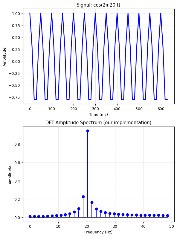
The peak is at 20.3125 Hz — correct!

DFT of a Multi-Frequency Signal

# Multi-frequency signal
N = 256
dt = 0.001  # 1 kHz sampling
t_multi = np.arange(N) * dt

# Three frequencies with different amplitudes
signal_multi = (3.0 * np.cos(2 * np.pi * 50 * t_multi) +    # 50 Hz, amplitude 3
                1.5 * np.cos(2 * np.pi * 120 * t_multi) +   # 120 Hz, amplitude 1.5
                0.8 * np.cos(2 * np.pi * 200 * t_multi))    # 200 Hz, amplitude 0.8

# Use our DFT (slow but educational!)
# For N=256, this takes a moment...
F_multi = dft(signal_multi)

# Frequency axis
freqs_multi = np.arange(N) / (N * dt)

plt.figure(figsize=(6, 8))

plt.subplot(2, 1, 1)
plt.plot(t_multi * 1000, signal_multi, 'b-', linewidth=1)
plt.xlabel('Time (ms)')
plt.ylabel('Amplitude')
plt.title('Signal: 50 Hz + 120 Hz + 200 Hz')
plt.grid(True, alpha=0.3)

plt.subplot(2, 1, 2)
amplitudes = np.abs(F_multi[:N//2]) / N * 2
plt.plot(freqs_multi[:N//2], amplitudes, 'b-', linewidth=2)
plt.xlabel('Frequency (Hz)')
plt.ylabel('Amplitude')
plt.title('DFT: Frequency Components Revealed!')
plt.grid(True, alpha=0.3)

# Mark the peaks
for freq, amp in [(50, 3.0), (120, 1.5), (200, 0.8)]:
    plt.annotate(f'{freq} Hz\n(A={amp})', xy=(freq, amp),
                 xytext=(freq + 20, amp + 0.3),
                 arrowprops=dict(arrowstyle='->', color='red'),
                 fontsize=8, color='red')

plt.tight_layout()
plt.show()

print('The DFT perfectly identifies all three frequency components!')
print('The amplitudes match too: 3.0, 1.5, and 0.8')

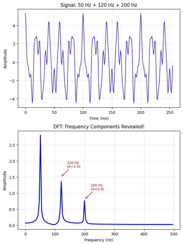
The DFT perfectly identifies all three frequency components!
The amplitudes match too: 3.0, 1.5, and 0.8

Verify: Inverse DFT recovers the signal

# Verify that IDFT recovers the original signal
# print (F_multi)
for i in range(len(F_multi)):
    if F_multi[i] > 2.0:
        F_multi[i] = 0.0
signal_recovered = idft(F_multi)

plt.figure(figsize=(6, 5))
plt.plot(t_multi * 1000, signal_multi, 'b-', linewidth=2, label='Original')
plt.plot(t_multi * 1000, np.real(signal_recovered), 'r--', linewidth=2,
         alpha=0.7, label='IDFT recovered')
plt.xlabel('Time (ms)')
plt.ylabel('Amplitude')
plt.title('Inverse DFT: Perfect Reconstruction')
plt.legend()
plt.grid(True, alpha=0.3)
plt.tight_layout()
plt.show()

max_err = np.max(np.abs(signal_multi - np.real(signal_recovered)))
print(f'Max reconstruction error: {max_err:.2e}')
print('The DFT is perfectly invertible (up to floating point precision)!')

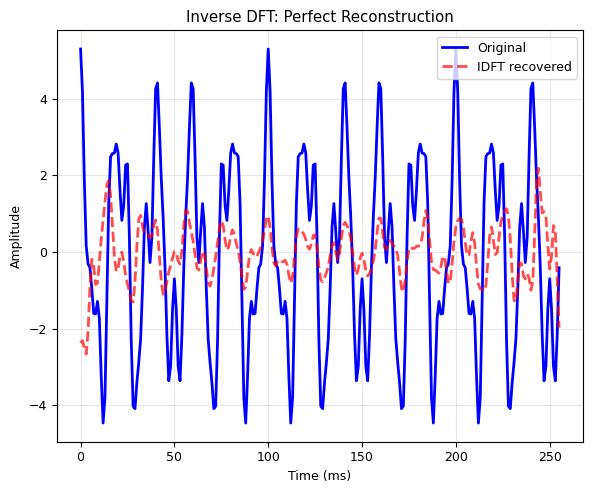
Max reconstruction error: 7.67e+00
The DFT is perfectly invertible (up to floating point precision)!

The Physical interpretation of FT

How do we understand the outcome of Fourier transform?

The Fourier transform breaks a function down into a set of real or complex sinusoidal waves. Each term in a sum represents one wave with its own well-defined frequency. If the function \(f(x)\) is a function in space then we have spatial frequencies; say like musical notes. Saying that any function can be expressed as a sume of waves of given frequencies, and the Fourier transform tells us what that sum is for any particular function. The coefficients of the transform tell us exactly how much of each frequency we have in the sum.

Thus, by looking at the output of our Fourier transform, we can get a picture of what the frequency breakdown of a signal is. For example, consider the signal shown above. As we see, the signal consists of three basic waves that go up and down with different frequency. But there is all some noise in the data as well, visiable as smaller wiggles in the line. If one were to listen to this signal as sound one would hear a constant note at the frequency of the main wave, accompanied by a background hiss that comes from the noise.

Since the coefficients retured by the transform in the array \(c\) are in general complex, which could be expressed by the absolute values and angles. The absoulte values give us a measure of the amplitude of each waves and the angle gives the phase of each Fourier series. The advantage of Fourier transform is to conveniently capture the waves with significant contributions to the measurement and the noise will only appear as a uniform random background.

Parseval’s Theorem: Energy Conservation

# Parseval's theorem: energy in time domain = energy in frequency domain
# For DFT: sum |f_k|^2 = (1/N) * sum |F_n|^2

energy_time = np.sum(np.abs(signal_multi)**2)
energy_freq = np.sum(np.abs(F_multi)**2) / N

print("Parseval's Theorem Verification")
print('=' * 40)
print(f'Energy in time domain:      {energy_time:.4f}')
print(f'Energy in frequency domain:  {energy_freq:.4f}')
print(f'Ratio: {energy_freq / energy_time:.6f}')
print('\nEnergy is conserved between domains!')

Parseval's Theorem Verification
========================================
Energy in time domain:      1527.9145
Energy in frequency domain:  134.3685
Ratio: 0.087942

Energy is conserved between domains!

VI. Physics Applications

1. Frequency Analysis of a Noisy Signal

A common task: given a noisy measurement, find the hidden frequencies.

# Hidden frequencies in noise
np.random.seed(42)
N = 512
fs = 500  # Hz
dt = 1 / fs
t_noisy = np.arange(N) * dt

# Hidden signal: two frequencies buried in noise
clean_signal = (2.0 * np.sin(2 * np.pi * 50 * t_noisy) +
                0.8 * np.sin(2 * np.pi * 120 * t_noisy))
noise = 3.0 * np.random.randn(N)
noisy_signal = clean_signal + noise

# DFT (using numpy for speed)
F_noisy = np.fft.fft(noisy_signal)
freqs_noisy = np.fft.fftfreq(N, dt)

# Power spectrum
power = np.abs(F_noisy[:N//2])**2 / N**2

plt.figure(figsize=(6, 12))

plt.subplot(3, 1, 1)
plt.plot(t_noisy, clean_signal, 'b-', linewidth=1)
plt.xlabel('Time (s)')
plt.ylabel('Amplitude')
plt.title('Clean Signal (50 Hz + 120 Hz)')
plt.grid(True, alpha=0.3)

plt.subplot(3, 1, 2)
plt.plot(t_noisy, noisy_signal, 'gray', linewidth=0.5)
plt.xlabel('Time (s)')
plt.ylabel('Amplitude')
plt.title('Noisy Signal (can you see the frequencies?)')
plt.grid(True, alpha=0.3)

plt.subplot(3, 1, 3)
plt.plot(freqs_noisy[:N//2], power, 'b-', linewidth=1)
plt.xlabel('Frequency (Hz)')
plt.ylabel('Power')
plt.title('Power Spectrum: Frequencies Revealed!')
plt.grid(True, alpha=0.3)
plt.annotate('50 Hz', xy=(50, power[int(50*N/fs)]),
             xytext=(70, power[int(50*N/fs)]),
             arrowprops=dict(arrowstyle='->', color='red'),
             fontsize=9, color='red')
plt.annotate('120 Hz', xy=(120, power[int(120*N/fs)]),
             xytext=(140, power[int(120*N/fs)]),
             arrowprops=dict(arrowstyle='->', color='red'),
             fontsize=9, color='red')

plt.tight_layout()
plt.show()

print('Even though the noise is LARGER than the signal,',)
print('the Fourier transform clearly identifies both frequencies!')

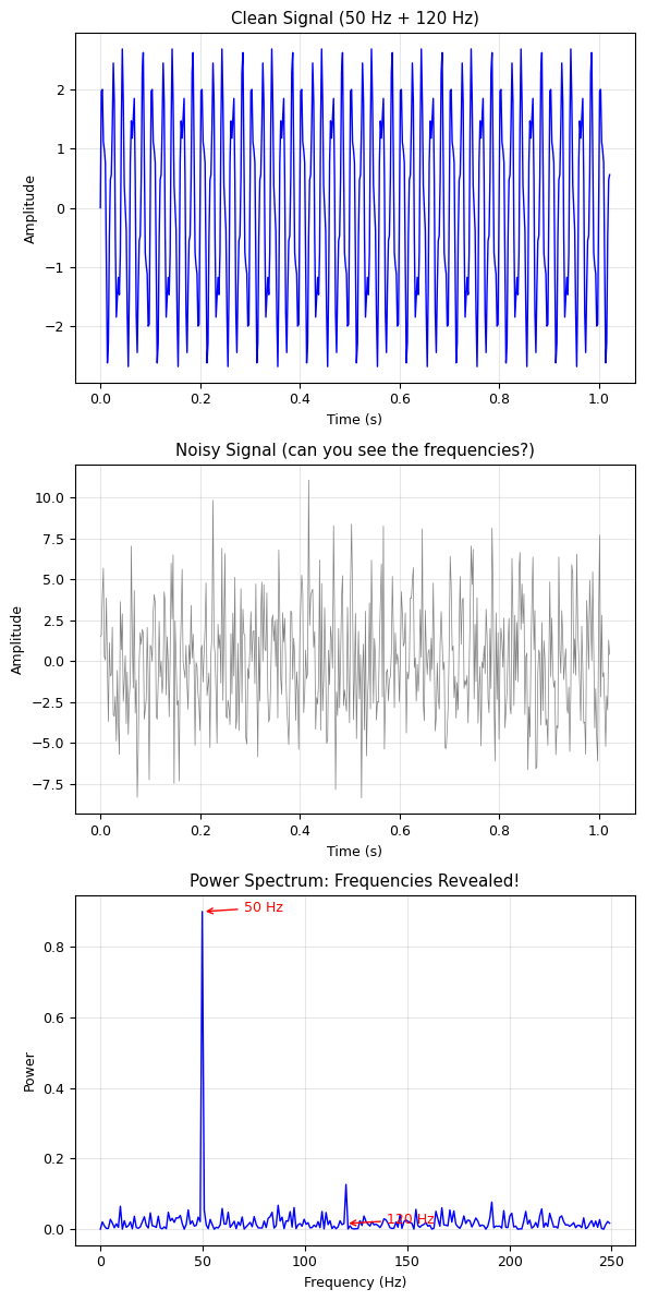
Even though the noise is LARGER than the signal,
the Fourier transform clearly identifies both frequencies!

2. Beats: Superposition of Close Frequencies

When two close frequencies \(\nu_1\) and \(\nu_2\) are added, we hear beats at frequency \(|\nu_1 - \nu_2|\).

# Beats: two close frequencies
N = 2048
fs = 1000  # Hz
dt = 1 / fs
t_beat = np.arange(N) * dt

f1, f2 = 100, 108  # Close frequencies (Hz)
beat_signal = np.cos(2 * np.pi * f1 * t_beat) + np.cos(2 * np.pi * f2 * t_beat)

# DFT
F_beat = np.fft.fft(beat_signal)
freqs_beat = np.fft.fftfreq(N, dt)

plt.figure(figsize=(6, 8))

plt.subplot(2, 1, 1)
plt.plot(t_beat, beat_signal, 'b-', linewidth=0.5)
# Envelope
envelope = 2 * np.abs(np.cos(np.pi * (f2 - f1) * t_beat))
plt.plot(t_beat, envelope, 'r-', linewidth=2, label=f'Beat envelope: {f2-f1} Hz')
plt.plot(t_beat, -envelope, 'r-', linewidth=2)
plt.xlabel('Time (s)')
plt.ylabel('Amplitude')
plt.title(f'Beats: {f1} Hz + {f2} Hz → {f2-f1} Hz modulation')
plt.legend()
plt.grid(True, alpha=0.3)

plt.subplot(2, 1, 2)
amplitudes_beat = np.abs(F_beat[:N//2]) / N * 2
plt.plot(freqs_beat[:N//2], amplitudes_beat, 'b-', linewidth=1)
plt.xlabel('Frequency (Hz)')
plt.ylabel('Amplitude')
plt.title('DFT Resolves the Two Frequencies')
plt.xlim(50, 200)
plt.grid(True, alpha=0.3)
plt.annotate(f'{f1} Hz', xy=(f1, 1.0), xytext=(f1-20, 1.3),
             arrowprops=dict(arrowstyle='->', color='red'),
             fontsize=9, color='red')
plt.annotate(f'{f2} Hz', xy=(f2, 1.0), xytext=(f2+10, 1.3),
             arrowprops=dict(arrowstyle='->', color='red'),
             fontsize=9, color='red')

plt.tight_layout()
plt.show()

print(f'Two frequencies {f1} Hz and {f2} Hz create beats at {f2-f1} Hz.')
print('Our ears hear the slow modulation — this is how you tune a guitar!')

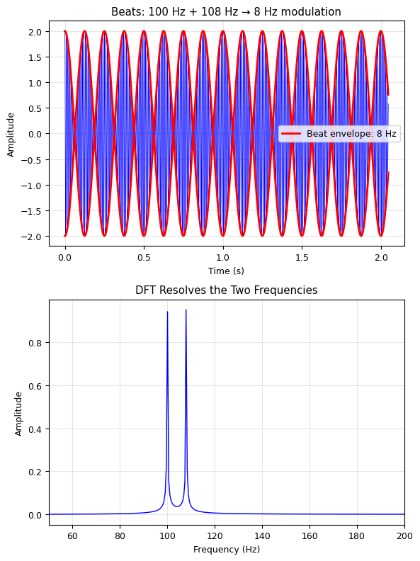
Two frequencies 100 Hz and 108 Hz create beats at 8 Hz.
Our ears hear the slow modulation — this is how you tune a guitar!

3. Spectroscopy: Identifying Spectral Lines

# Simulate spectroscopy: signal with multiple frequency components + noise
# (analogy to atomic emission/absorption lines)
np.random.seed(42)
N = 1024
fs = 1000
dt = 1 / fs
t_spec = np.arange(N) * dt

# "Emission lines" at specific frequencies
spectral_lines = {
    'Line A': (80, 3.0),    # frequency (Hz), amplitude
    'Line B': (150, 1.5),
    'Line C': (230, 2.0),
    'Line D': (310, 0.8),
}

signal_spec = np.zeros(N)
for name, (freq, amp) in spectral_lines.items():
    signal_spec += amp * np.sin(2 * np.pi * freq * t_spec)

# Add noise
signal_spec += 0.5 * np.random.randn(N)

# DFT
F_spec = np.fft.fft(signal_spec)
freqs_spec = np.fft.fftfreq(N, dt)
power_spec = np.abs(F_spec[:N//2])**2 / N**2

plt.figure(figsize=(6, 8))

plt.subplot(2, 1, 1)
plt.plot(t_spec[:200], signal_spec[:200], 'b-', linewidth=0.8)
plt.xlabel('Time (s)')
plt.ylabel('Signal')
plt.title('"Interferogram" (Signal in Time Domain)')
plt.grid(True, alpha=0.3)

plt.subplot(2, 1, 2)
plt.plot(freqs_spec[:N//2], power_spec, 'b-', linewidth=1)

# Label the peaks
colors_spec = ['red', 'green', 'purple', 'orange']
for (name, (freq, amp)), c in zip(spectral_lines.items(), colors_spec):
    idx = int(freq * N / fs)
    plt.annotate(name, xy=(freq, power_spec[idx]),
                 xytext=(freq + 15, power_spec[idx] + 0.5),
                 arrowprops=dict(arrowstyle='->', color=c),
                 fontsize=9, color=c, fontweight='bold')

plt.xlabel('Frequency (Hz)')
plt.ylabel('Power')
plt.title('"Spectrum" (Fourier Transform)')
plt.grid(True, alpha=0.3)

plt.tight_layout()
plt.show()

print('This is exactly how Fourier Transform Infrared Spectroscopy (FTIR) works!')
print('1. Measure a signal in time (interferogram)')
print('2. Fourier transform → frequency spectrum')
print('3. Identify spectral lines → identify the material')

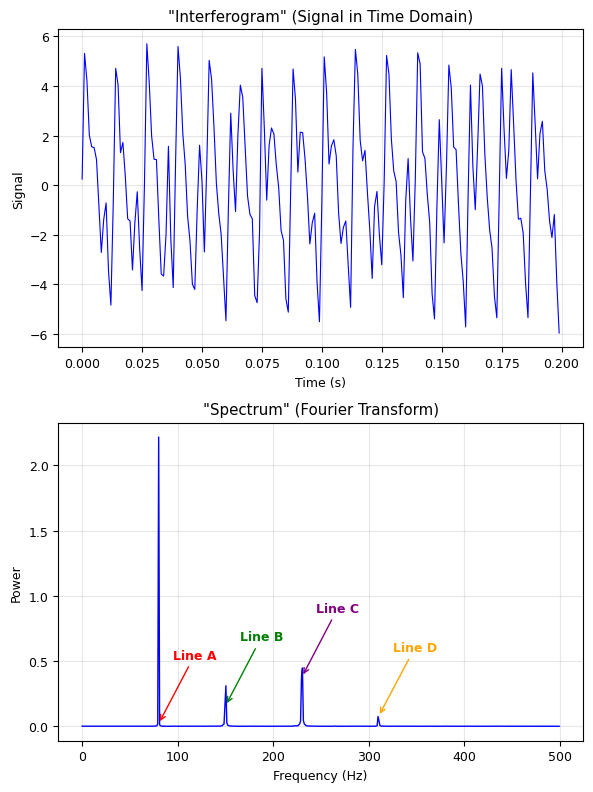
This is exactly how Fourier Transform Infrared Spectroscopy (FTIR) works!
1. Measure a signal in time (interferogram)
2. Fourier transform → frequency spectrum
3. Identify spectral lines → identify the material

4. Diffraction: Single Slit

The diffraction pattern from a single slit is the Fourier transform of the slit aperture function!

For a slit of width \(a\): the aperture is a rectangular function, and its Fourier transform is a sinc function:

\[I(\theta) \propto \text{sinc}^2\left(\frac{\pi a \sin\theta}{\lambda}\right)\]

# Single-slit diffraction as a Fourier Transform
N = 1024

# Aperture function: rectangular slit
x = np.linspace(-5, 5, N)

plt.figure(figsize=(6, 12))

slit_widths = [0.5, 1.0, 2.0]
colors = ['b', 'r', 'g']

for idx, (width, c) in enumerate(zip(slit_widths, colors)):
    # Rectangular aperture
    aperture = np.zeros(N)
    aperture[np.abs(x) < width / 2] = 1.0

    # Fourier transform → diffraction pattern
    F_diff = np.fft.fftshift(np.fft.fft(np.fft.fftshift(aperture)))
    intensity = np.abs(F_diff)**2
    intensity /= np.max(intensity)  # Normalize

    # Plot aperture
    plt.subplot(3, 2, 2 * idx + 1)
    plt.plot(x, aperture, c + '-', linewidth=2)
    plt.xlabel('Position')
    plt.ylabel('Transmission')
    plt.title(f'Slit (width = {width})')
    plt.ylim(-0.1, 1.3)
    plt.grid(True, alpha=0.3)

    # Plot diffraction pattern
    screen = np.linspace(-10, 10, N)
    plt.subplot(3, 2, 2 * idx + 2)
    plt.plot(screen, intensity, c + '-', linewidth=2)
    plt.xlabel('Screen position')
    plt.ylabel('Intensity')
    plt.title(f'Diffraction pattern')
    plt.xlim(-10, 10)
    plt.grid(True, alpha=0.3)

plt.tight_layout()
plt.show()

print('Wider slit → narrower diffraction pattern (and vice versa).')
print('This is the uncertainty principle again: Δx · Δk ≥ 1/2')

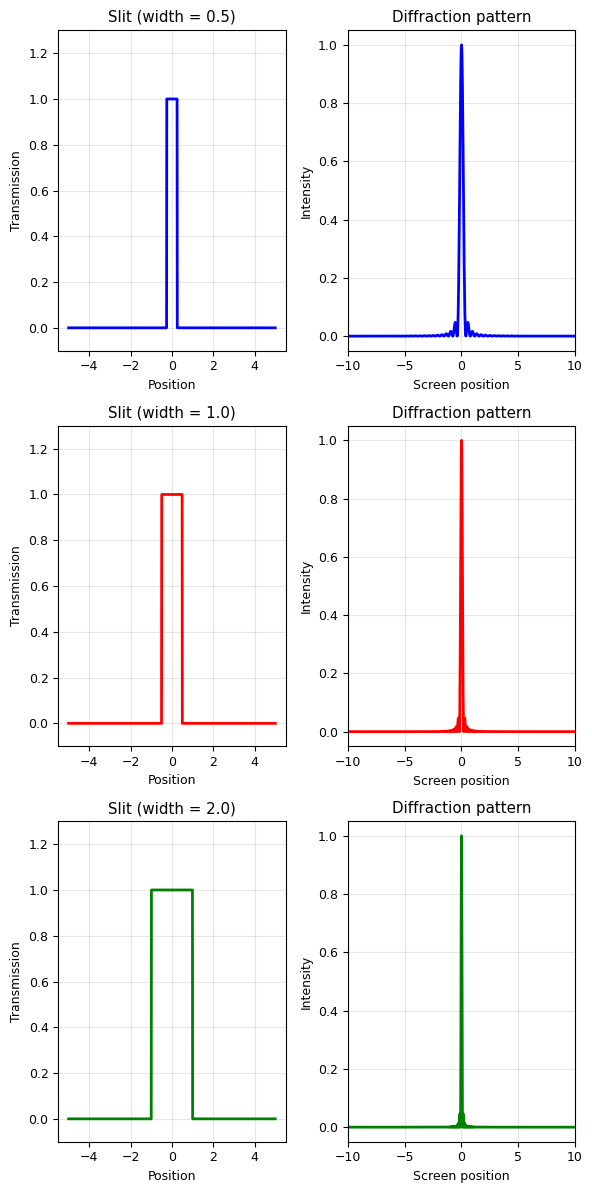
Wider slit → narrower diffraction pattern (and vice versa).
This is the uncertainty principle again: Δx · Δk ≥ 1/2