Lecture 21 — Machine Learning II

Lecture 21 — Machine Learning II#

Neural Networks & Deep Learning#

Computational Physics — Spring 2026

From Logistic Regression to Neural Networks#

In Lecture 20, logistic regression computed:

\[ \hat{y} = \sigma(\mathbf{w}^T \mathbf{x} + b) \]

This is a single neuron: it takes inputs, computes a weighted sum, and passes it through a non-linear activation function $\sigma$.

A neural network is simply many neurons organised in layers. By stacking layers, the network can learn arbitrarily complex functions — this is the universal approximation theorem.

import numpy as np
import matplotlib.pyplot as plt

plt.rcParams['figure.figsize'] = [6, 4]
plt.rcParams['font.size'] = 9

print("Ready for Neural Networks!")

Ready for Neural Networks!

I. Anatomy of a Neural Network#

The Single Neuron (Perceptron)#

A single neuron computes:

\[ \text{output} = \phi\!\left(\sum_{j=1}^{n} w_j x_j + b\right) = \phi(\mathbf{w}^T \mathbf{x} + b) \]

where $\phi$ is a non-linear activation function.

Without $\phi$, stacking layers would just give another linear transformation — the non-linearity is essential.

# Common activation functions
z = np.linspace(-4, 4, 300)

activations = {
    'Sigmoid': 1 / (1 + np.exp(-z)),
    'Tanh': np.tanh(z),
    'ReLU': np.maximum(0, z),
    'Leaky ReLU': np.where(z > 0, z, 0.1 * z),
}

fig, axes = plt.subplots(1, 4, figsize=(14, 3))
for ax, (name, values) in zip(axes, activations.items()):
    ax.plot(z, values, 'b-', lw=2)
    ax.axhline(0, color='gray', ls='--', alpha=0.3)
    ax.axvline(0, color='gray', ls='--', alpha=0.3)
    ax.set_title(name)
    ax.set_xlabel('z')
    ax.grid(alpha=0.2)

plt.tight_layout()
plt.show()

print("Modern networks almost always use ReLU or its variants.")
print("Sigmoid/tanh suffer from 'vanishing gradients' in deep networks.")

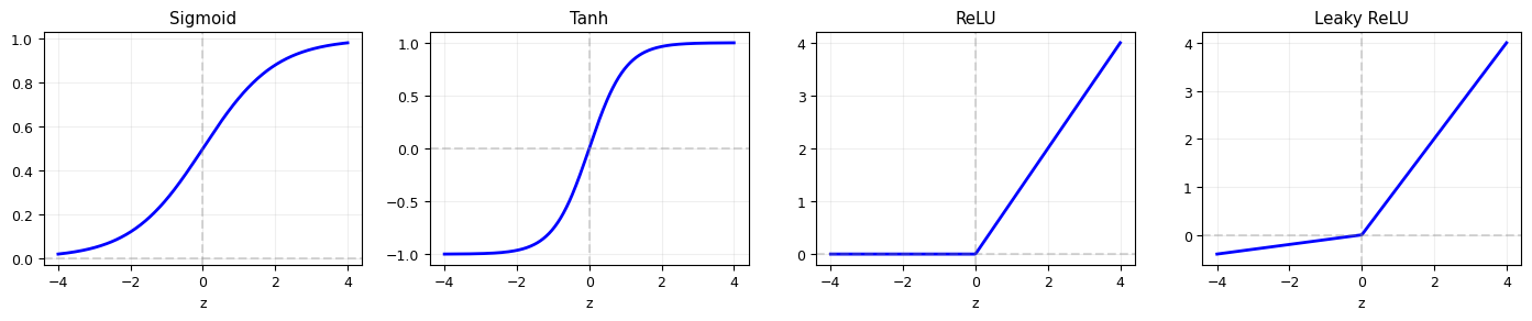
_images/3265ec47ca69c4dbb924b727f8067a4afda57ea0213eb8b4909197fc31ac32e2.png

Modern networks almost always use ReLU or its variants.
Sigmoid/tanh suffer from 'vanishing gradients' in deep networks.

Multi-Layer Perceptron (MLP)#

An MLP stacks neurons in layers:

Input (d features)  →  Hidden layer 1 (h₁ neurons)  →  Hidden layer 2 (h₂ neurons)  →  Output
     x₁, x₂, ...          φ(W₁x + b₁)                    φ(W₂h₁ + b₂)                ŷ

Mathematically, a 2-hidden-layer MLP computes:

\[ \hat{y} = \mathbf{W}_3 \,\phi\!\bigl(\mathbf{W}_2 \,\phi(\mathbf{W}_1 \mathbf{x} + \mathbf{b}_1) + \mathbf{b}_2\bigr) + \mathbf{b}_3 \]

Parameters: All the weight matrices $\mathbf{W}_l$ and bias vectors $\mathbf{b}_l$.

A network with $d$ inputs, one hidden layer of $h$ neurons, and 1 output has $(d+1)h + (h+1) = (d+2)h + 1$ parameters.

Universal Approximation Theorem#

A feedforward network with a single hidden layer containing a finite number of neurons can approximate any continuous function on a compact subset of $\mathbb{R}^n$, to arbitrary accuracy. — Cybenko (1989), Hornik (1991)

This tells us neural networks are expressive enough in principle. But it says nothing about:

How many neurons we need (could be exponentially many)
Whether gradient descent can find the right weights
Whether the network will generalise

In practice, deeper networks (more layers) are more efficient than wider ones, which is why we use “deep” learning.

II. Building a Neural Network from Scratch#

Before using PyTorch, let’s implement a simple 2-layer MLP manually to understand every step.

# A minimal neural network from scratch (numpy only)
# Task: learn the function f(x) = sin(x) on [0, 2pi]

np.random.seed(42)

# Training data
N = 100
x_data = np.random.uniform(0, 2*np.pi, N)
y_data = np.sin(x_data)

# Normalise inputs (zero mean, unit variance)
# Without this, ~half the ReLU neurons are dead at initialisation
# because x > 0 always and b starts at 0
x_mean, x_std = x_data.mean(), x_data.std()
x_norm = (x_data - x_mean) / x_std

# Network architecture: 1 input -> 32 hidden (ReLU) -> 1 output
n_hidden = 32

# Initialise weights (He initialisation)
W1 = np.random.randn(1, n_hidden) * np.sqrt(2.0 / 1)    # (1, 32)
b1 = np.zeros((1, n_hidden))                              # (1, 32)
W2 = np.random.randn(n_hidden, 1) * np.sqrt(2.0 / n_hidden)  # (32, 1)
b2 = np.zeros((1, 1))                                     # (1, 1)

print(f"Parameters: W1 {W1.shape}, b1 {b1.shape}, W2 {W2.shape}, b2 {b2.shape}")
print(f"Total parameters: {W1.size + b1.size + W2.size + b2.size}")

Parameters: W1 (1, 32), b1 (1, 32), W2 (32, 1), b2 (1, 1)
Total parameters: 97

def relu(z):
    return np.maximum(0, z)

def relu_grad(z):
    return (z > 0).astype(float)

def forward(x, W1, b1, W2, b2):
    """Forward pass: input → hidden → output."""
    z1 = x @ W1 + b1     # pre-activation of hidden layer
    a1 = relu(z1)         # activation of hidden layer
    z2 = a1 @ W2 + b2    # output (linear, no activation for regression)
    return z1, a1, z2

def mse_loss(y_pred, y_true):
    """Mean squared error."""
    return np.mean((y_pred - y_true) ** 2)

print("Forward pass and loss defined.")

Forward pass and loss defined.

Backpropagation = Chain Rule#

To update the weights, we need $\partial L / \partial \mathbf{W}_l$ for each layer. Backpropagation computes these using the chain rule, working backwards from the loss:

\[ \frac{\partial L}{\partial \mathbf{W}_2} = \mathbf{a}_1^T \, \delta_2 \qquad\text{where}\quad \delta_2 = \frac{\partial L}{\partial \mathbf{z}_2} = \frac{2}{N}(\hat{y} - y) \]

\[ \frac{\partial L}{\partial \mathbf{W}_1} = \mathbf{x}^T \, \delta_1 \qquad\text{where}\quad \delta_1 = (\delta_2 \, \mathbf{W}_2^T) \odot \phi'(\mathbf{z}_1) \]

This is just the gradient descent from Lecture 15, applied to a more complex function!

# Training loop with backpropagation
X = x_norm.reshape(-1, 1)  # (N, 1) — normalised inputs
Y = y_data.reshape(-1, 1)  # (N, 1)

lr = 0.01   # learning rate
losses = []

for epoch in range(10000):
    # Forward pass
    z1, a1, z2 = forward(X, W1, b1, W2, b2)
    y_pred = z2
    loss = mse_loss(y_pred, Y)
    losses.append(loss)

    # Backward pass
    delta2 = 2.0 / N * (y_pred - Y)        # (N, 1)
    dW2 = a1.T @ delta2                     # (32, 1)
    db2 = np.sum(delta2, axis=0, keepdims=True)  # (1, 1)

    delta1 = (delta2 @ W2.T) * relu_grad(z1)  # (N, 32)
    dW1 = X.T @ delta1                      # (1, 32)
    db1 = np.sum(delta1, axis=0, keepdims=True)  # (1, 32)

    # Gradient descent update (Lecture 15!)
    W2 -= lr * dW2
    b2 -= lr * db2
    W1 -= lr * dW1
    b1 -= lr * db1

    if epoch % 1000 == 0:
        print(f"Epoch {epoch:4d}  Loss: {loss:.6f}")

print(f"Final loss: {losses[-1]:.6f}")

Epoch    0  Loss: 0.003822
Epoch 1000  Loss: 0.002310
Epoch 2000  Loss: 0.001570
Epoch 3000  Loss: 0.001145
Epoch 4000  Loss: 0.000879
Epoch 5000  Loss: 0.000701
Epoch 6000  Loss: 0.000574
Epoch 7000  Loss: 0.000477
Epoch 8000  Loss: 0.000406
Epoch 9000  Loss: 0.000340
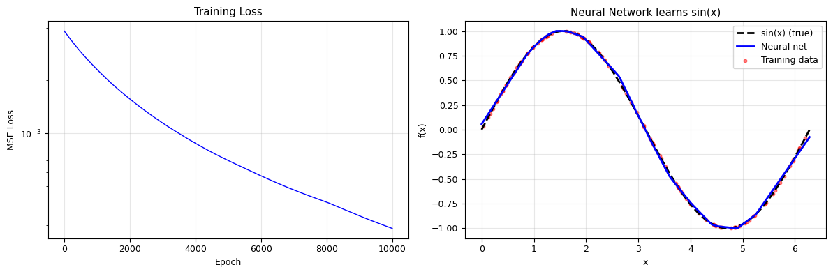
Final loss: 0.000288

# Visualise the result
fig, axes = plt.subplots(1, 2, figsize=(12, 4))

# Loss curve
axes[0].semilogy(losses, 'b-', lw=1)
axes[0].set_xlabel('Epoch')
axes[0].set_ylabel('MSE Loss')
axes[0].set_title('Training Loss')
axes[0].grid(alpha=0.3)

# Prediction vs truth
x_plot = np.linspace(0, 2*np.pi, 300)
x_plot_norm = ((x_plot - x_mean) / x_std).reshape(-1, 1)
_, _, y_plot = forward(x_plot_norm, W1, b1, W2, b2)

axes[1].plot(x_plot, np.sin(x_plot), 'k--', lw=2, label='sin(x) (true)')
axes[1].plot(x_plot, y_plot, 'b-', lw=2, label='Neural net')
axes[1].scatter(x_data, y_data, c='red', s=10, alpha=0.5, label='Training data')
axes[1].set_xlabel('x'); axes[1].set_ylabel('f(x)')
axes[1].set_title('Neural Network learns sin(x)')
axes[1].legend()
axes[1].grid(alpha=0.3)

plt.tight_layout()
plt.show()

_images/835de2f15883db0eca901bb5f9a89c6bb70f2562e2ef0c5bb439a067b493cba8.png

III. PyTorch: Automatic Differentiation#

Writing backpropagation by hand is tedious and error-prone. PyTorch provides:

Tensors — like NumPy arrays but can track gradients
Autograd — automatic differentiation (computes all gradients for you)
nn.Module — building blocks for neural networks
Optimisers — SGD, Adam, etc.

PyTorch builds a computational graph during the forward pass and uses it to compute gradients automatically during the backward pass.

import torch
import torch.nn as nn

print(f"PyTorch version: {torch.__version__}")
print(f"CUDA available: {torch.cuda.is_available()}")
device = 'cuda' if torch.cuda.is_available() else 'cpu'
print(f"Using device: {device}")

PyTorch version: 2.10.0+cpu
CUDA available: False
Using device: cpu

# PyTorch autograd demo
# Compute gradient of f(x) = x^3 + 2x at x = 3
# Analytical: f'(x) = 3x^2 + 2 => f'(3) = 29

x = torch.tensor(3.0, requires_grad=True)
f = x**3 + 2*x
f.backward()  # compute df/dx

print(f"f(3) = {f.item():.1f}")
print(f"f'(3) = {x.grad.item():.1f}  (analytical: 29.0)")
print("\nPyTorch computed the gradient automatically!")

f(3) = 33.0
f'(3) = 29.0  (analytical: 29.0)

PyTorch computed the gradient automatically!

Building an MLP with `nn.Module`#

class MLP(nn.Module):
    """Simple Multi-Layer Perceptron."""

    def __init__(self, input_dim, hidden_dims, output_dim):
        super().__init__()
        layers = []
        prev_dim = input_dim
        for h in hidden_dims:
            layers.append(nn.Linear(prev_dim, h))
            layers.append(nn.ReLU())
            prev_dim = h
        layers.append(nn.Linear(prev_dim, output_dim))
        self.net = nn.Sequential(*layers)

    def forward(self, x):
        return self.net(x)

# Create a network: 1 input → [64, 64] hidden → 1 output
model = MLP(input_dim=1, hidden_dims=[64, 64], output_dim=1)

# Count parameters
n_params = sum(p.numel() for p in model.parameters())
print(f"Network architecture:\n{model}")
print(f"\nTotal parameters: {n_params}")

Network architecture:
MLP(
  (net): Sequential(
    (0): Linear(in_features=1, out_features=64, bias=True)
    (1): ReLU()
    (2): Linear(in_features=64, out_features=64, bias=True)
    (3): ReLU()
    (4): Linear(in_features=64, out_features=1, bias=True)
  )
)

Total parameters: 4353

# Training loop in PyTorch
torch.manual_seed(42)

# Data
X_t = torch.tensor(x_data, dtype=torch.float32).reshape(-1, 1)
Y_t = torch.tensor(y_data, dtype=torch.float32).reshape(-1, 1)

# Model, loss, optimiser
model = MLP(1, [64, 64], 1)
criterion = nn.MSELoss()
optimizer = torch.optim.Adam(model.parameters(), lr=0.01)

# Train
losses_pt = []
for epoch in range(1000):
    optimizer.zero_grad()            # clear old gradients
    y_pred = model(X_t)              # forward pass
    loss = criterion(y_pred, Y_t)    # compute loss
    loss.backward()                  # backward pass (autograd!)
    optimizer.step()                 # update weights
    losses_pt.append(loss.item())

    if epoch % 200 == 0:
        print(f"Epoch {epoch:4d}  Loss: {loss.item():.6f}")

print(f"Final loss: {losses_pt[-1]:.6f}")

Epoch    0  Loss: 0.418733
Epoch  200  Loss: 0.000130
Epoch  400  Loss: 0.000088
Epoch  600  Loss: 0.000016
Epoch  800  Loss: 0.000007
Final loss: 0.000007

# Compare: numpy from scratch vs PyTorch
fig, axes = plt.subplots(1, 2, figsize=(12, 4))

# Loss comparison
axes[0].semilogy(losses, 'r-', alpha=0.7, label='NumPy (from scratch)')
axes[0].semilogy(losses_pt, 'b-', alpha=0.7, label='PyTorch (Adam)')
axes[0].set_xlabel('Epoch')
axes[0].set_ylabel('MSE Loss')
axes[0].set_title('Training convergence')
axes[0].legend()
axes[0].grid(alpha=0.3)

# PyTorch prediction
x_plot_t = torch.linspace(0, 2*np.pi, 300).reshape(-1, 1)
with torch.no_grad():
    y_plot_t = model(x_plot_t).numpy()

axes[1].plot(x_plot_t.numpy(), np.sin(x_plot_t.numpy()), 'k--', lw=2, label='sin(x)')
axes[1].plot(x_plot_t.numpy(), y_plot_t, 'b-', lw=2, label='PyTorch MLP')
axes[1].scatter(x_data, y_data, c='red', s=10, alpha=0.5)
axes[1].set_title('PyTorch MLP learns sin(x)')
axes[1].legend()
axes[1].grid(alpha=0.3)

plt.tight_layout()
plt.show()

print("PyTorch + Adam converges much faster than manual SGD!")

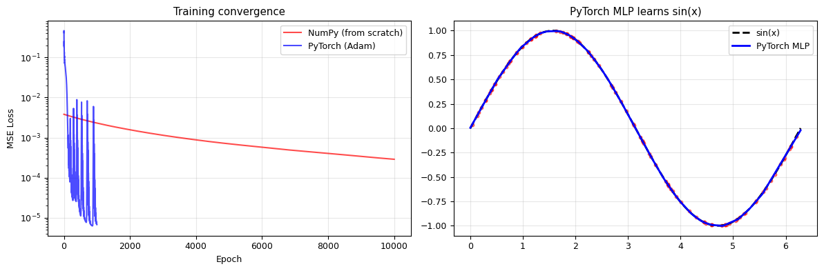
_images/fd106a62add7a634798d42c288359b967051a0649493139ff68825166f262c3e.png

PyTorch + Adam converges much faster than manual SGD!

IV. Training in Practice#

Key Concepts#

Loss Functions#

Task	Loss	PyTorch
Regression	MSE: $\frac{1}{N}\sum(y-\hat{y})^2$	`nn.MSELoss()`
Regression	MAE: $\frac{1}{N}\sum	y-\hat{y}
Binary classification	Cross-entropy	`nn.BCEWithLogitsLoss()`
Multi-class	Cross-entropy	`nn.CrossEntropyLoss()`

Optimisers#

Optimiser	Key idea	When to use
SGD	Basic gradient descent (Lecture 15)	Baseline, large-scale
SGD + momentum	Accumulate velocity	Faster convergence
Adam	Adaptive learning rate per parameter	Default choice
AdamW	Adam + weight decay	When regularisation matters

Mini-Batch Training#

For large datasets, computing the gradient over all $N$ samples is expensive. Instead, we use mini-batches:

Split data into batches of size $B$ (typically 32–256)
Compute gradient on each batch → update weights
One pass through all batches = one epoch

This is stochastic gradient descent (SGD) — the gradient is noisy but the noise actually helps escape local minima (recall Monte Carlo / Lecture 14).

from torch.utils.data import TensorDataset, DataLoader

# Create a DataLoader for mini-batch training
dataset = TensorDataset(X_t, Y_t)
loader = DataLoader(dataset, batch_size=16, shuffle=True)

print(f"Dataset size: {len(dataset)}")
print(f"Batch size: 16")
print(f"Batches per epoch: {len(loader)}")

# One epoch of mini-batch training
for batch_x, batch_y in loader:
    print(f"  Batch shape: {batch_x.shape}")
    break  # just show the first batch

Dataset size: 100
Batch size: 16
Batches per epoch: 7
  Batch shape: torch.Size([16, 1])

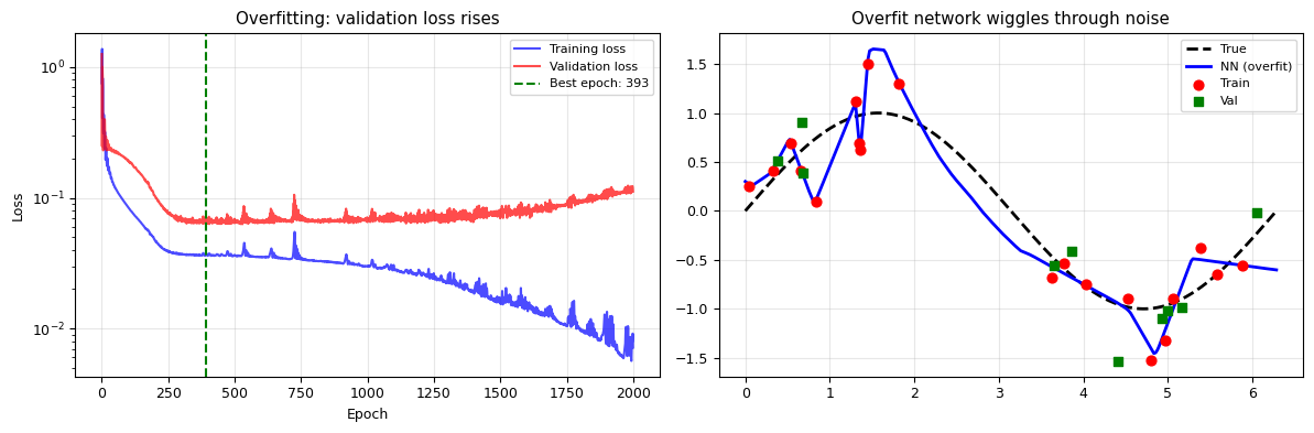
Overfitting and Regularisation in Neural Networks#

Neural networks can have millions of parameters — they can memorise training data perfectly. Common regularisation techniques:

Early stopping: Stop training when validation loss starts increasing
Weight decay (L2 regularisation): Add $\lambda\|\mathbf{w}\|^2$ to loss
Dropout: Randomly set neurons to zero during training
Data augmentation: Create synthetic training examples

# Demo: Overfitting and early stopping
torch.manual_seed(42)

# Small noisy dataset — easy to overfit
N_small = 30
x_small = np.random.uniform(0, 2*np.pi, N_small)
y_small = np.sin(x_small) + 0.3 * np.random.randn(N_small)

# Split into train/val
X_tr = torch.tensor(x_small[:20], dtype=torch.float32).reshape(-1, 1)
Y_tr = torch.tensor(y_small[:20], dtype=torch.float32).reshape(-1, 1)
X_val = torch.tensor(x_small[20:], dtype=torch.float32).reshape(-1, 1)
Y_val = torch.tensor(y_small[20:], dtype=torch.float32).reshape(-1, 1)

# Big model (easy to overfit with 20 data points)
model_big = MLP(1, [128, 128], 1)
optimizer = torch.optim.Adam(model_big.parameters(), lr=0.005)
criterion = nn.MSELoss()

train_losses, val_losses = [], []
for epoch in range(2000):
    model_big.train()
    optimizer.zero_grad()
    loss_tr = criterion(model_big(X_tr), Y_tr)
    loss_tr.backward()
    optimizer.step()

    model_big.eval()
    with torch.no_grad():
        loss_val = criterion(model_big(X_val), Y_val)

    train_losses.append(loss_tr.item())
    val_losses.append(loss_val.item())

# Plot
fig, axes = plt.subplots(1, 2, figsize=(12, 4))

axes[0].semilogy(train_losses, 'b-', label='Training loss', alpha=0.7)
axes[0].semilogy(val_losses, 'r-', label='Validation loss', alpha=0.7)
best_epoch = np.argmin(val_losses)
axes[0].axvline(best_epoch, color='green', ls='--', label=f'Best epoch: {best_epoch}')
axes[0].set_xlabel('Epoch'); axes[0].set_ylabel('Loss')
axes[0].set_title('Overfitting: validation loss rises')
axes[0].legend(fontsize=8); axes[0].grid(alpha=0.3)

# Prediction at final epoch vs what it should be
x_plot_t = torch.linspace(0, 2*np.pi, 300).reshape(-1, 1)
with torch.no_grad():
    y_plot_big = model_big(x_plot_t).numpy()

axes[1].plot(x_plot_t.numpy(), np.sin(x_plot_t.numpy()), 'k--', lw=2, label='True')
axes[1].plot(x_plot_t.numpy(), y_plot_big, 'b-', lw=2, label='NN (overfit)')
axes[1].scatter(x_small[:20], y_small[:20], c='red', s=40, zorder=5, label='Train')
axes[1].scatter(x_small[20:], y_small[20:], c='green', s=40, zorder=5, marker='s', label='Val')
axes[1].set_title('Overfit network wiggles through noise')
axes[1].legend(fontsize=8); axes[1].grid(alpha=0.3)

plt.tight_layout()
plt.show()

_images/1a881fbfb2ca20ed92fbf83da353ef608eb85d0ea2460fdc83bd2c5d1bbb255e.png

V. Physics Application: Learning a Potential Energy Surface#

In computational physics and chemistry, we often need the potential energy $V(\mathbf{r})$ as a function of atomic positions. Computing this from first principles (DFT, ab initio) is expensive. Can a neural network learn the potential energy surface from training data?

The Lennard-Jones Potential#

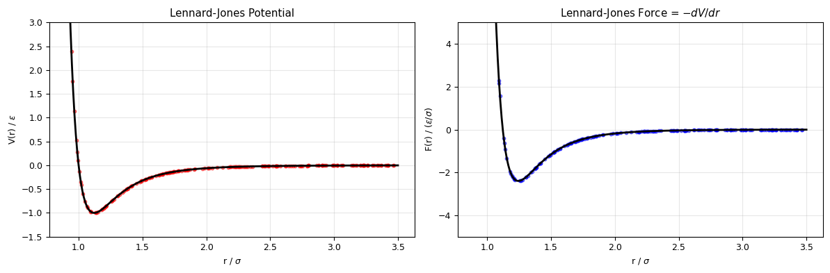
As a test case, we use the Lennard-Jones pair potential:

\[ V(r) = 4\varepsilon \left[ \left(\frac{\sigma}{r}\right)^{12} - \left(\frac{\sigma}{r}\right)^6 \right] \]

For a cluster of $N$ atoms, the total energy is:

\[ E_{\text{total}} = \sum_{i<j} V(r_{ij}) \]

We will train a neural network to predict $V(r)$ and its derivative (the force $F = -dV/dr$) simultaneously.

# Lennard-Jones potential and force
def lj_potential(r, epsilon=1.0, sigma=1.0):
    """Lennard-Jones potential."""
    sr6 = (sigma / r) ** 6
    return 4 * epsilon * (sr6**2 - sr6)

def lj_force(r, epsilon=1.0, sigma=1.0):
    """LJ force = -dV/dr."""
    sr6 = (sigma / r) ** 6
    return 4 * epsilon * (12 * sr6**2 / r - 6 * sr6 / r)

# Generate training data
np.random.seed(42)
r_train = np.random.uniform(0.9, 3.5, 200)
V_train = lj_potential(r_train)
F_train = lj_force(r_train)

# Visualise
r_plot = np.linspace(0.9, 3.5, 500)
fig, axes = plt.subplots(1, 2, figsize=(12, 4))

axes[0].plot(r_plot, lj_potential(r_plot), 'k-', lw=2)
axes[0].scatter(r_train, V_train, c='red', s=10, alpha=0.5)
axes[0].set_xlabel('r / $\\sigma$'); axes[0].set_ylabel('V(r) / $\\varepsilon$')
axes[0].set_title('Lennard-Jones Potential')
axes[0].set_ylim(-1.5, 3); axes[0].grid(alpha=0.3)

axes[1].plot(r_plot, lj_force(r_plot), 'k-', lw=2)
axes[1].scatter(r_train, F_train, c='blue', s=10, alpha=0.5)
axes[1].set_xlabel('r / $\\sigma$'); axes[1].set_ylabel('F(r) / ($\\varepsilon / \\sigma$)')
axes[1].set_title('Lennard-Jones Force = $-dV/dr$')
axes[1].set_ylim(-5, 5); axes[1].grid(alpha=0.3)

plt.tight_layout()
plt.show()

_images/08ac9dbea45880fc5598d423879484fdacc1ab67aede17b65f3f0f2887d07c71.png

Training a Neural Network Potential#

We train a network to predict $V(r)$, but we also want it to predict the correct force $F = -dV/dr$.

Key trick: use PyTorch’s autograd to compute $-dV_{\text{NN}}/dr$ and include it in the loss:

\[ L = \underbrace{\sum_i (V_{\text{NN}}(r_i) - V_{\text{true}}(r_i))^2}_{\text{energy loss}} + \lambda \underbrace{\sum_i (F_{\text{NN}}(r_i) - F_{\text{true}}(r_i))^2}_{\text{force loss}} \]

This is a preview of physics-informed training (Lecture 23).

# Neural network potential with force matching
torch.manual_seed(42)

class NNPotential(nn.Module):
    """Neural network that predicts energy and force."""
    def __init__(self):
        super().__init__()
        self.net = nn.Sequential(
            nn.Linear(1, 64),
            nn.Tanh(),
            nn.Linear(64, 64),
            nn.Tanh(),
            nn.Linear(64, 1),
        )

    def forward(self, r):
        return self.net(r)

    def energy_and_force(self, r):
        """Compute energy and force (via autograd)."""
        r.requires_grad_(True)
        V = self.forward(r)
        # Force = -dV/dr, computed by autograd
        F = -torch.autograd.grad(
            V.sum(), r, create_graph=True
        )[0]
        return V, F

nn_pot = NNPotential()
n_params = sum(p.numel() for p in nn_pot.parameters())
print(f"NN Potential: {n_params} parameters")

NN Potential: 4353 parameters

# Prepare data as tensors
r_t = torch.tensor(r_train, dtype=torch.float32).reshape(-1, 1)
V_t = torch.tensor(V_train, dtype=torch.float32).reshape(-1, 1)
F_t = torch.tensor(F_train, dtype=torch.float32).reshape(-1, 1)

optimizer = torch.optim.Adam(nn_pot.parameters(), lr=0.005)
force_weight = 1.0  # relative weight of force loss

losses_energy, losses_force = [], []

for epoch in range(3000):
    optimizer.zero_grad()

    V_pred, F_pred = nn_pot.energy_and_force(r_t.clone())

    loss_E = nn.MSELoss()(V_pred, V_t)
    loss_F = nn.MSELoss()(F_pred, F_t)
    loss = loss_E + force_weight * loss_F

    loss.backward()
    optimizer.step()

    losses_energy.append(loss_E.item())
    losses_force.append(loss_F.item())

    if epoch % 600 == 0:
        print(f"Epoch {epoch:4d}  Energy loss: {loss_E.item():.6f}  Force loss: {loss_F.item():.6f}")

print(f"\nFinal — Energy loss: {losses_energy[-1]:.6f}, Force loss: {losses_force[-1]:.6f}")

Epoch    0  Energy loss: 0.396379  Force loss: 178.423416
Epoch  600  Energy loss: 0.000025  Force loss: 0.008059
Epoch 1200  Energy loss: 0.000022  Force loss: 0.004959
Epoch 1800  Energy loss: 0.000016  Force loss: 0.003905
Epoch 2400  Energy loss: 0.000477  Force loss: 0.141569

Final — Energy loss: 0.000006, Force loss: 0.002581

# Evaluate the trained NN potential
r_test = torch.linspace(0.9, 3.5, 500).reshape(-1, 1)
nn_pot.eval()
V_nn, F_nn = nn_pot.energy_and_force(r_test.clone())
V_nn = V_nn.detach().numpy()
F_nn = F_nn.detach().numpy()

fig, axes = plt.subplots(1, 3, figsize=(15, 4))

# Energy
axes[0].plot(r_test.numpy(), lj_potential(r_test.numpy()), 'k--', lw=2, label='True LJ')
axes[0].plot(r_test.numpy(), V_nn, 'b-', lw=2, label='NN potential')
axes[0].set_xlabel('r / $\\sigma$'); axes[0].set_ylabel('V(r)')
axes[0].set_title('Potential Energy')
axes[0].set_ylim(-1.5, 3); axes[0].legend(); axes[0].grid(alpha=0.3)

# Force
axes[1].plot(r_test.numpy(), lj_force(r_test.numpy()), 'k--', lw=2, label='True force')
axes[1].plot(r_test.numpy(), F_nn, 'r-', lw=2, label='NN force (autograd)')
axes[1].set_xlabel('r / $\\sigma$'); axes[1].set_ylabel('F(r)')
axes[1].set_title('Force = $-dV/dr$')
axes[1].set_ylim(-5, 5); axes[1].legend(); axes[1].grid(alpha=0.3)

# Training curves
axes[2].semilogy(losses_energy, 'b-', alpha=0.7, label='Energy loss')
axes[2].semilogy(losses_force, 'r-', alpha=0.7, label='Force loss')
axes[2].set_xlabel('Epoch'); axes[2].set_ylabel('MSE')
axes[2].set_title('Training progress')
axes[2].legend(); axes[2].grid(alpha=0.3)

plt.tight_layout()
plt.show()

print("The NN learns both the potential AND the correct forces!")
print("The force comes 'for free' via automatic differentiation.")

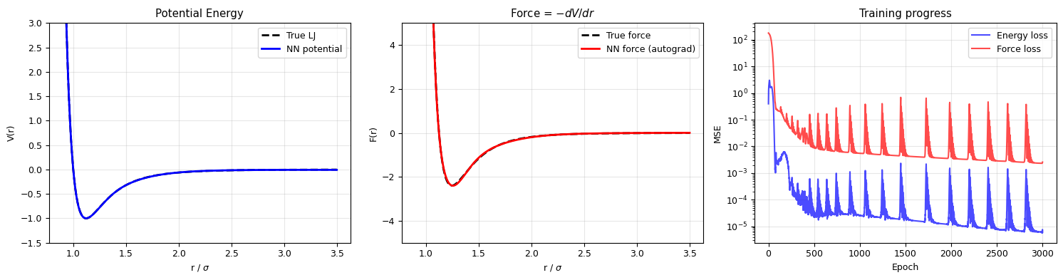
_images/52ab9f995b4cb34e29c03a0d9530bde39bc6635c3903684e5e7dedd45c3c91ee.png

The NN learns both the potential AND the correct forces!
The force comes 'for free' via automatic differentiation.

VI. Multi-Atom System: LJ Cluster Energy#

Now let’s predict the total energy of a small cluster of atoms, where the energy depends on all pairwise distances.

def lj_cluster_energy(positions, epsilon=1.0, sigma=1.0):
    """Total LJ energy for a cluster of atoms.
    positions: (N_atoms, 3) array
    """
    N = len(positions)
    E = 0.0
    for i in range(N):
        for j in range(i+1, N):
            r = np.linalg.norm(positions[i] - positions[j])
            E += lj_potential(r, epsilon, sigma)
    return E

def get_pairwise_distances(positions):
    """Compute all pairwise distances (sorted) as features."""
    N = len(positions)
    dists = []
    for i in range(N):
        for j in range(i+1, N):
            dists.append(np.linalg.norm(positions[i] - positions[j]))
    return np.sort(dists)  # sorted for permutation invariance

# Generate random 4-atom clusters and compute their energies
np.random.seed(42)
n_samples = 2000
n_atoms = 4
n_pairs = n_atoms * (n_atoms - 1) // 2  # = 6 pairwise distances

X_cluster = []
E_cluster = []

for _ in range(n_samples):
    # Random positions near the equilibrium distance
    pos = np.random.randn(n_atoms, 3) * 0.8
    dists = get_pairwise_distances(pos)

    # Skip configurations with atoms too close
    if dists.min() < 0.8:
        continue

    E = lj_cluster_energy(pos)
    X_cluster.append(dists)
    E_cluster.append(E)

X_cluster = np.array(X_cluster)
E_cluster = np.array(E_cluster)

print(f"Generated {len(X_cluster)} valid configurations")
print(f"Features per sample: {n_pairs} pairwise distances")
print(f"Energy range: [{E_cluster.min():.2f}, {E_cluster.max():.2f}]")

Generated 1262 valid configurations
Features per sample: 6 pairwise distances
Energy range: [-4.20, 77.49]

# Train NN to predict cluster energy from pairwise distances
from sklearn.model_selection import train_test_split as tts

X_tr, X_te, E_tr, E_te = tts(X_cluster, E_cluster, test_size=0.2, random_state=42)

# Standardise
X_mean, X_std = X_tr.mean(axis=0), X_tr.std(axis=0)
E_mean, E_std = E_tr.mean(), E_tr.std()

X_tr_n = (X_tr - X_mean) / X_std
X_te_n = (X_te - X_mean) / X_std
E_tr_n = (E_tr - E_mean) / E_std
E_te_n = (E_te - E_mean) / E_std

# Tensors
X_tr_t = torch.tensor(X_tr_n, dtype=torch.float32)
E_tr_t = torch.tensor(E_tr_n, dtype=torch.float32).reshape(-1, 1)
X_te_t = torch.tensor(X_te_n, dtype=torch.float32)
E_te_t = torch.tensor(E_te_n, dtype=torch.float32).reshape(-1, 1)

# Train
torch.manual_seed(42)
cluster_model = MLP(n_pairs, [128, 128, 64], 1)
optimizer = torch.optim.Adam(cluster_model.parameters(), lr=0.002)
criterion = nn.MSELoss()

loader = DataLoader(TensorDataset(X_tr_t, E_tr_t), batch_size=64, shuffle=True)

train_l, val_l = [], []
for epoch in range(300):
    cluster_model.train()
    epoch_loss = 0
    for bx, by in loader:
        optimizer.zero_grad()
        loss = criterion(cluster_model(bx), by)
        loss.backward()
        optimizer.step()
        epoch_loss += loss.item()
    train_l.append(epoch_loss / len(loader))

    cluster_model.eval()
    with torch.no_grad():
        val_l.append(criterion(cluster_model(X_te_t), E_te_t).item())

    if epoch % 60 == 0:
        print(f"Epoch {epoch:3d}  Train: {train_l[-1]:.5f}  Val: {val_l[-1]:.5f}")

print(f"Final val loss: {val_l[-1]:.5f}")

Epoch   0  Train: 0.79955  Val: 0.82202
Epoch  60  Train: 0.00539  Val: 0.05320
Epoch 120  Train: 0.00759  Val: 0.04778
Epoch 180  Train: 0.01588  Val: 0.04999
Epoch 240  Train: 0.02666  Val: 0.07756
Final val loss: 0.04686

# Parity plot: predicted vs true energy
cluster_model.eval()
with torch.no_grad():
    E_pred_n = cluster_model(X_te_t).numpy().flatten()

# Un-standardise
E_pred = E_pred_n * E_std + E_mean

fig, axes = plt.subplots(1, 2, figsize=(12, 5))

# Parity plot
axes[0].scatter(E_te, E_pred, s=10, alpha=0.5)
emin, emax = min(E_te.min(), E_pred.min()), max(E_te.max(), E_pred.max())
axes[0].plot([emin, emax], [emin, emax], 'r--', lw=2, label='Perfect')
axes[0].set_xlabel('True Energy ($\\varepsilon$)')
axes[0].set_ylabel('Predicted Energy ($\\varepsilon$)')
axes[0].set_title('Parity Plot: NN vs True')
axes[0].legend(); axes[0].grid(alpha=0.3)

# Error distribution
errors = E_pred - E_te
axes[1].hist(errors, bins=40, edgecolor='black', alpha=0.7)
axes[1].set_xlabel('Prediction Error ($\\varepsilon$)')
axes[1].set_ylabel('Count')
axes[1].set_title(f'Error Distribution (MAE = {np.abs(errors).mean():.4f})')
axes[1].axvline(0, color='red', ls='--')

plt.tight_layout()
plt.show()

from sklearn.metrics import r2_score
print(f"R² score: {r2_score(E_te, E_pred):.4f}")
print(f"MAE: {np.abs(errors).mean():.4f} epsilon")

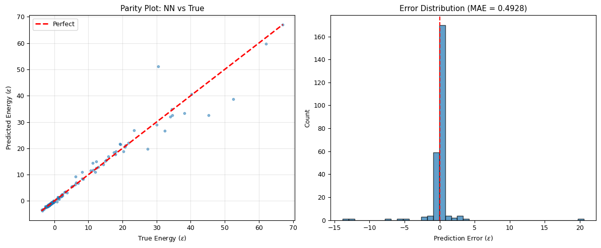
_images/0e8a14d4fecb7bdfcf0197f5202973d457a18bef029bae46c24589afc037bc96.png

R² score: 0.9652
MAE: 0.4928 epsilon

VII. Ising Model Revisited: NN Classifier#

Let’s revisit the Ising phase classification from Lecture 21, now using a neural network.

# Generate Ising data (same as Lecture 21)
def metropolis_ising(L, T, n_sweeps=1000, n_equil=500):
    spins = np.random.choice([-1, 1], size=(L, L))
    beta = 1.0 / T
    configs = []
    for sweep in range(n_sweeps):
        for _ in range(L * L):
            i, j = np.random.randint(0, L, size=2)
            neighbours = (
                spins[(i+1) % L, j] + spins[(i-1) % L, j] +
                spins[i, (j+1) % L] + spins[i, (j-1) % L]
            )
            dE = 2 * spins[i, j] * neighbours
            if dE <= 0 or np.random.rand() < np.exp(-beta * dE):
                spins[i, j] *= -1
        if sweep >= n_equil and sweep % 10 == 0:
            configs.append(spins.copy())
    return configs

L = 16
T_c = 2.269
temperatures = np.concatenate([np.linspace(1.0, 2.0, 6), np.linspace(2.5, 4.0, 6)])

X_ising, y_ising = [], []
print("Generating Ising data...")
for T in temperatures:
    configs = metropolis_ising(L, T, n_sweeps=2000, n_equil=1000)
    for cfg in configs:
        X_ising.append(cfg.flatten().astype(np.float32))
        y_ising.append(0 if T < T_c else 1)

X_ising = np.array(X_ising)
y_ising = np.array(y_ising)
print(f"Dataset: {len(X_ising)} samples, {X_ising.shape[1]} features")

Generating Ising data...
Dataset: 1200 samples, 256 features

# Split and convert to tensors
X_tr, X_te, y_tr, y_te = tts(X_ising, y_ising, test_size=0.3, random_state=42)

X_tr_t = torch.tensor(X_tr, dtype=torch.float32)
y_tr_t = torch.tensor(y_tr, dtype=torch.long)
X_te_t = torch.tensor(X_te, dtype=torch.float32)
y_te_t = torch.tensor(y_te, dtype=torch.long)

# NN classifier
torch.manual_seed(42)

class IsingClassifier(nn.Module):
    def __init__(self, input_dim):
        super().__init__()
        self.net = nn.Sequential(
            nn.Linear(input_dim, 64),
            nn.ReLU(),
            nn.Dropout(0.2),
            nn.Linear(64, 32),
            nn.ReLU(),
            nn.Linear(32, 2),  # 2 classes
        )

    def forward(self, x):
        return self.net(x)

ising_nn = IsingClassifier(L * L)
optimizer = torch.optim.Adam(ising_nn.parameters(), lr=0.001)
criterion = nn.CrossEntropyLoss()

loader = DataLoader(TensorDataset(X_tr_t, y_tr_t), batch_size=32, shuffle=True)

# Train
for epoch in range(50):
    ising_nn.train()
    for bx, by in loader:
        optimizer.zero_grad()
        loss = criterion(ising_nn(bx), by)
        loss.backward()
        optimizer.step()

    if epoch % 10 == 0:
        ising_nn.eval()
        with torch.no_grad():
            pred_tr = ising_nn(X_tr_t).argmax(dim=1)
            pred_te = ising_nn(X_te_t).argmax(dim=1)
            acc_tr = (pred_tr == y_tr_t).float().mean().item()
            acc_te = (pred_te == y_te_t).float().mean().item()
        print(f"Epoch {epoch:2d}  Train acc: {acc_tr:.3f}  Test acc: {acc_te:.3f}")

# Final accuracy
ising_nn.eval()
with torch.no_grad():
    final_acc = (ising_nn(X_te_t).argmax(dim=1) == y_te_t).float().mean().item()
print(f"\nFinal test accuracy: {final_acc:.3f}")

Epoch  0  Train acc: 0.924  Test acc: 0.919
Epoch 10  Train acc: 1.000  Test acc: 0.981
Epoch 20  Train acc: 1.000  Test acc: 0.981
Epoch 30  Train acc: 1.000  Test acc: 0.978
Epoch 40  Train acc: 1.000  Test acc: 0.986

Final test accuracy: 0.967

Summary#

Concept	Key Idea
Neuron	Weighted sum + non-linear activation
MLP	Stack neurons in layers
Activation functions	ReLU (modern default), sigmoid, tanh
Backpropagation	Chain rule on the computational graph
PyTorch	Automatic differentiation + GPU acceleration
Loss functions	MSE (regression), cross-entropy (classification)
Adam optimiser	Adaptive learning rates — the default choice
Overfitting	Early stopping, dropout, weight decay
NN potentials	Learn $V(r)$ and get forces $F = -dV/dr$ via autograd

Task	Loss	PyTorch
Regression	MSE: \(\frac{1}{N}\sum(y-\hat{y})^2\)	`nn.MSELoss()`
Regression	MAE: $\frac{1}{N}\sum	y-\hat{y}
Binary classification	Cross-entropy	`nn.BCEWithLogitsLoss()`
Multi-class	Cross-entropy	`nn.CrossEntropyLoss()`