Lecture 12: Stochastic Methods I#
Computational Physics — Spring 2026
Stochastic Methods I: The Art of Randomness#
Introduction to Randomness in Physics#
Nature is filled with phenomena that exhibit random or seemingly random behavior. From the unpredictable decay of radioactive nuclei to the erratic Brownian motion of particles suspended in a fluid, randomness is deeply embedded in the fabric of physical reality. These stochastic processes play a crucial role in various fields:
Quantum mechanics: The inherently probabilistic nature of quantum measurements
Statistical mechanics: Random molecular motions underlying thermodynamic properties
Astrophysics: Random stellar formations and galaxy distributions
Biological physics: Random fluctuations in cellular processes
To model these phenomena computationally, we need reliable methods to generate random numbers. But this raises an interesting paradox: how can we create randomness using deterministic computers?
import numpy as np
import matplotlib.pyplot as plt
from scipy import special, stats
from scipy.ndimage import label

plt.rcParams['figure.figsize'] = [6, 4]
plt.rcParams['font.size'] = 9

print("Ready for stochastic adventures!")
Ready for stochastic adventures!
I. Random Numbers and Distributions#
Pseudo-Random Number Generation#
True randomness is difficult to achieve on a computer. Instead, we use algorithms that produce sequences of numbers that appear random but are actually generated by deterministic formulas. These are called pseudo-random number generators (PRNGs).
A good PRNG should have:
Long periods before repeating sequences
Statistical properties resembling true randomness
Efficiency in computation
Reproducibility when needed (for debugging)
Linear Congruential Generator (LCG)#
The Linear Congruential Generator (LCG) is one of the simplest and most historically significant PRNGs. Despite its simplicity, it illustrates the fundamental principles behind most modern random number generators.
Mathematical Foundation:
The LCG is based on the following recursive formula:
Where:
\(X_n\) is the current number in the sequence
\(X_{n+1}\) is the next number in the sequence
\(a\), \(c\), and \(m\) are carefully chosen integer constants
\(X_0\) is the initial value, called the “seed”
This formula generates a sequence of integers between 0 and \(m-1\).
Key Properties:
Deterministic: Given the same parameters and seed, the sequence will always be identical
Periodic: The sequence will eventually repeat with a maximum period of \(m\)
Parameter-sensitive: The quality of randomness critically depends on the choice of \(a\), \(c\), and \(m\)
Let’s examine a basic implementation:
N = 100  # Number of random numbers to generate
a = 1111  # Multiplier
c = 1000 # Increment
m = 130    # Modulus
x = 3     # Initial seed
results = []

for i in range(N):
    x = (a*x + c) % m
    results.append(x)

print(results)

plt.plot(results, "o")
plt.title("Random Number Sequence from LCG")
plt.xlabel("Iteration")
plt.ylabel("Random Value")
plt.grid(alpha=0.3)
plt.show()
[43, 23, 33, 93, 63, 13, 103, 123, 113, 53, 83, 3, 43, 23, 33, 93, 63, 13, 103, 123, 113, 53, 83, 3, 43, 23, 33, 93, 63, 13, 103, 123, 113, 53, 83, 3, 43, 23, 33, 93, 63, 13, 103, 123, 113, 53, 83, 3, 43, 23, 33, 93, 63, 13, 103, 123, 113, 53, 83, 3, 43, 23, 33, 93, 63, 13, 103, 123, 113, 53, 83, 3, 43, 23, 33, 93, 63, 13, 103, 123, 113, 53, 83, 3, 43, 23, 33, 93, 63, 13, 103, 123, 113, 53, 83, 3, 43, 23, 33, 93]
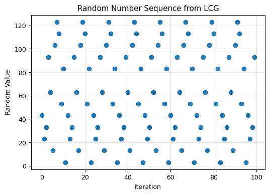
As shown above, we calculated the first 100 numbers in the sequence generated by the LCG equation with parameters \(\{a, c, m\}\). The generated numbers appear to be quite random.
This is a linear congruential random number generator, which generates a string of random integers by iterating the same equation many times. It is the most fundamental way of generating random numbers on a computer.
Key observations:
The numbers are not truly random. If you know the values of \(\{a, c, m\}\) plus the seed, you can exactly predict the sequence. Using the same parameters always gives the same output.
The numbers are always non-negative (between 0 and \(m-1\)).
The results are very sensitive to the choice of \(\{a, c, m\}\). For example, if both \(c\) and \(m\) are even, the generator would only produce even or only odd numbers. It is wise to use only values which have been thoroughly tested.
For a particular set of \(\{a, c, m\}\), you can still get different sequences by varying the initial value of \(X_0\). This initial value is called the seed of the random number generator.
Provided that one is aware of these conditions, the linear congruential generator can be used to produce pseudo-random numbers for simple calculations. In practice, modern libraries like NumPy use far more sophisticated algorithms (e.g., the Mersenne Twister with period \(2^{19937}-1\)).
LCG as a Python Class and Function#
For better usability, we can encapsulate the LCG algorithm in a class or a standalone function:
class LCG:
    def __init__(self, seed, a, c, m):
        self.state = seed
        self.a = a
        self.c = c
        self.m = m

    def next_random(self):
        self.state = (self.a * self.state + self.c) % self.m
        return self.state
# Standalone function version
def lcg(seed, a, c, m):
    """One step of a Linear Congruential Generator."""
    r = (a * seed + c) % m
    return r

seed = 12
a = 3330   # Multiplier
c = 1630   # Increment
m = 13     # Modulus

r1 = lcg(seed, a, c, m)
print(f"seed={seed} -> r1={r1}")

r2 = lcg(r1, a, c, m)
print(f"r1={r1}   -> r2={r2}")

r3 = lcg(r2, a, c, m)
print(f"r2={r2}   -> r3={r3}")
seed=12 -> r1=3
r1=3   -> r2=11
r2=11   -> r3=1
# Class version — maintains internal state
lcg_gen = LCG(seed=14, a=16231, c=1012, m=13)

for i in range(5):
    r = lcg_gen.next_random()
    print(f"Step {i+1}: {r}")
Step 1: 5
Step 2: 7
Step 3: 8
Step 4: 2
Step 5: 12
Generating Random Numbers in a Range#
To generate a random number in a specific range [min_value, max_value], we can normalize the output of the LCG and then scale it to the desired range.
class LCG:
    def __init__(self, seed, a, c, m):
        self.state = seed
        self.a = a
        self.c = c
        self.m = m

    def next_random(self):
        self.state = (self.a * self.state + self.c) % self.m
        return self.state

    def random(self):
        """Return a random float in (0, 1)."""
        return self.next_random()/self.m

    def randint(self, min_value, max_value):
        """Return a random integer in [min_value, max_value)."""
        return int(self.random() * (max_value-min_value) + min_value)


lcg = LCG(seed=1, a=1234, c=567, m=13)

print("Random integers in [-5, 5):")
for i in range(10):
    print(f"  {lcg.randint(-5, 5)}", end="")
print()

print("\nRandom integers in [100, 200):")
for i in range(10):
    print(f"  {lcg.randint(100, 200)}", end="")
print()

print("\nRandom floats in (0, 1):")
for i in range(10):
    print(f"  {lcg.random():.4f}", end="")
print()
Random integers in [-5, 5):
  0  -4  0  -4  0  -4  0  -4  0  -4

Random integers in [100, 200):
  153  107  153  107  153  107  153  107  153  107

Random floats in (0, 1):
  0.5385  0.0769  0.5385  0.0769  0.5385  0.0769  0.5385  0.0769  0.5385  0.0769
Critical Analysis of LCG Properties#
Pseudo-randomness: Despite appearing random, the sequence is entirely deterministic. Given the parameters and seed, anyone can predict every number in the sequence.
Value Range: The raw LCG output is always between 0 and \(m-1\), inclusive. This is important to consider when scaling to different ranges.
Parameter Sensitivity: The quality of randomness critically depends on the choice of parameters:
If both \(c\) and \(m\) are even, the sequence will alternate between even and odd numbers or get stuck in even worse patterns
Poor parameter choices can lead to very short periods
Some combinations create strong correlations between consecutive numbers
Seed Dependence: Different seeds produce different sequences, but the quality characteristics remain determined by the main parameters.
Periodicity: All LCGs eventually repeat their sequences. The maximum theoretical period is \(m\), but many parameter combinations result in much shorter periods.
The Art of Choosing Parameters#
The choice of parameters \(\{a, c, m\}\) is crucial and non-trivial. After decades of mathematical analysis, certain values have been proven to yield optimal results.
Hull-Dobell Theorem: For a full period (\(m\) values before repeating), the following must hold:
\(c\) and \(m\) are relatively prime
\(a-1\) is divisible by all prime factors of \(m\)
If \(m\) is divisible by 4, then \(a-1\) is also divisible by 4
An excellent and well-tested choice for 32-bit computers is:
\(a = 7^5 = 16807\)
\(c = 0\)
\(m = 2^{31} - 1 = 2{,}147{,}483{,}647\)
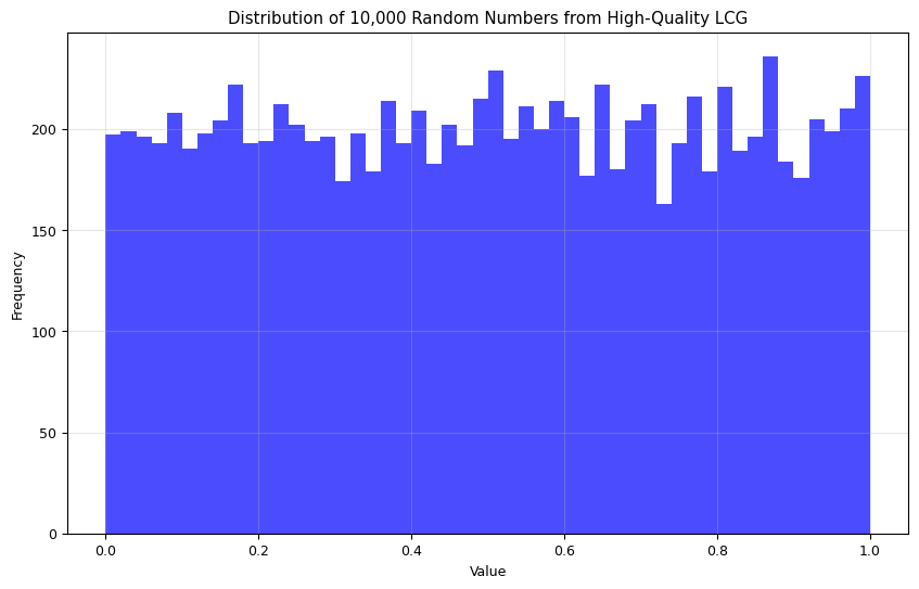
These parameters create a multiplicative congruential generator (a special case of LCG where \(c=0\)) that passes many statistical tests for randomness and has an impressively long period.
# Let's demonstrate the high-quality parameters
lcg = LCG(seed=1, a=16807, c=0, m=2**31-1)
### random seed, (year + month + day + hour + min + second ) (import time )
# Generate a large sample of random numbers
samples = [lcg.random() for _ in range(10000)]
# Plot histogram to check distribution
plt.figure(figsize=(10, 6))
plt.hist(samples, bins=50, alpha=0.7, color='blue')
plt.title('Distribution of 10,000 Random Numbers from High-Quality LCG')
plt.xlabel('Value')
plt.ylabel('Frequency')
plt.grid(alpha=0.3)
plt.show()
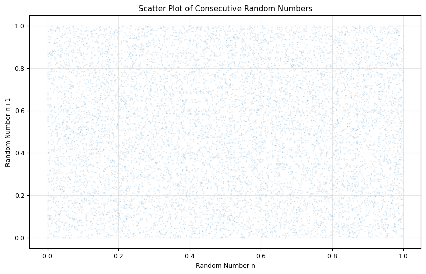
# Plot scatter to check for patterns between consecutive numbers
plt.figure(figsize=(10, 6))
plt.scatter(samples[:-1], samples[1:], alpha=0.1, s=1)
plt.title('Scatter Plot of Consecutive Random Numbers')
plt.xlabel('Random Number n')
plt.ylabel('Random Number n+1')
plt.grid(alpha=0.3)
plt.show()
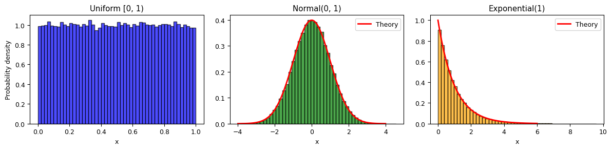
NumPy Random Number Tools#
In practice, we use NumPy’s well-tested random number generators rather than writing our own. NumPy uses the Mersenne Twister algorithm by default — far superior to a simple LCG.
Key functions:
np.random.seed(n): Set the seed for reproducibilitynp.random.uniform(0, 1, N): N uniform [0,1) samplesnp.random.normal(μ, σ, N): N Gaussian samplesnp.random.exponential(λ, N): N exponential samples
np.random.seed(42)

N = 100000
uniform_samples = np.random.uniform(0, 1, N)
normal_samples = np.random.normal(0, 1, N)
exponential_samples = np.random.exponential(1, N)

print("Uniform [0,1):")
print(f"  Mean: {np.mean(uniform_samples):.4f} (expected 0.5)")
print(f"  Std:  {np.std(uniform_samples):.4f} (expected {1/np.sqrt(12):.4f})")

print("\nNormal(mu=0, sigma=1):")
print(f"  Mean: {np.mean(normal_samples):.4f} (expected 0)")
print(f"  Std:  {np.std(normal_samples):.4f} (expected 1)")

print("\nExponential(lambda=1):")
print(f"  Mean: {np.mean(exponential_samples):.4f} (expected 1)")
print(f"  Std:  {np.std(exponential_samples):.4f} (expected 1)")
Uniform [0,1):
  Mean: 0.4995 (expected 0.5)
  Std:  0.2883 (expected 0.2887)

Normal(mu=0, sigma=1):
  Mean: 0.0026 (expected 0)
  Std:  0.9983 (expected 1)

Exponential(lambda=1):
  Mean: 1.0002 (expected 1)
  Std:  1.0018 (expected 1)
fig, axes = plt.subplots(1, 3, figsize=(12, 3))

axes[0].hist(uniform_samples, bins=50, density=True, alpha=0.7, color='blue', edgecolor='black')
axes[0].set_title('Uniform [0, 1)')
axes[0].set_xlabel('x')
axes[0].set_ylabel('Probability density')

axes[1].hist(normal_samples, bins=50, density=True, alpha=0.7, color='green', edgecolor='black')
x_gauss = np.linspace(-4, 4, 100)
axes[1].plot(x_gauss, stats.norm.pdf(x_gauss), 'r-', lw=2, label='Theory')
axes[1].set_title('Normal(0, 1)')
axes[1].set_xlabel('x')
axes[1].legend()

axes[2].hist(exponential_samples, bins=50, density=True, alpha=0.7, color='orange', edgecolor='black')
x_exp = np.linspace(0, 6, 100)
axes[2].plot(x_exp, np.exp(-x_exp), 'r-', lw=2, label='Theory')
axes[2].set_title('Exponential(1)')
axes[2].set_xlabel('x')
axes[2].legend()

plt.tight_layout()
plt.show()
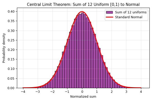
Central Limit Theorem: Sums of Uniforms → Gaussian#
Remarkable fact: The sum of many independent random variables approaches a Gaussian distribution, regardless of the shape of the original distribution.
Experiment: Take the sum of \(N\) uniform [0,1) random variables. Subtract the mean (\(N/2\)) and divide by the standard deviation (\(\sqrt{N/12}\)). The result converges to a standard normal as \(N\) grows!
np.random.seed(123)

N_uniform = 12
N_samples = 100000

sums = np.sum(np.random.uniform(0, 1, (N_samples, N_uniform)), axis=1)
sums_normalized = (sums - N_uniform/2) / np.sqrt(N_uniform/12)

fig, ax = plt.subplots(figsize=(6, 4))
ax.hist(sums_normalized, bins=50, density=True, alpha=0.7, color='purple', edgecolor='black', label=f'Sum of {N_uniform} uniforms')

x = np.linspace(-4, 4, 100)
ax.plot(x, stats.norm.pdf(x), 'r-', lw=2.5, label='Standard Normal')
ax.set_xlabel('Normalized sum')
ax.set_ylabel('Probability density')
ax.set_title('Central Limit Theorem: Sum of 12 Uniform [0,1) to Normal')
ax.legend()
ax.grid(alpha=0.3)
plt.tight_layout()
plt.show()
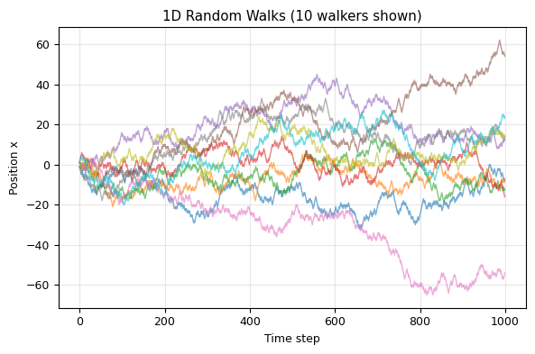
II. Random Walks and Diffusion#
1D Random Walk: Step Left or Right#
At each time step, a particle moves left (-1) or right (+1) with equal probability.
Key results:
Mean x = 0 (by symmetry)
Mean x^2 = N (after N steps)
Standard deviation: sigma ~ sqrt(N) (diffusive scaling)
Connection to physics: This is the microscopic origin of diffusion! The random walk in the continuum limit becomes the heat equation: d(rho)/dt = D d^2(rho)/dx^2
np.random.seed(111)

n_walkers = 100
n_steps = 1000

steps = np.random.choice([-1, 1], size=(n_walkers, n_steps))
positions = np.cumsum(steps, axis=1)

fig, ax = plt.subplots(figsize=(6, 4))
for i in range(min(10, n_walkers)):
    ax.plot(positions[i, :], alpha=0.6, lw=1)

ax.set_xlabel('Time step')
ax.set_ylabel('Position x')
ax.set_title(f'1D Random Walks ({min(10, n_walkers)} walkers shown)')
ax.grid(alpha=0.3)
plt.tight_layout()
plt.show()
final_positions = positions[:, -1]
final_positions_squared = final_positions**2

mean_x2 = np.mean(final_positions_squared)
expected_x2 = n_steps

print(f"After N = {n_steps} steps:")
print(f"<x^2> observed: {mean_x2:.0f}")
print(f"<x^2> expected: {expected_x2:.0f}")
print(f"<x>:          {np.mean(final_positions):.2f} (should be approx 0)")
print(f"std(x):       {np.std(final_positions):.1f} approx sqrt({n_steps}) = {np.sqrt(n_steps):.1f}")

fig, ax = plt.subplots(figsize=(6, 4))
ax.hist(final_positions, bins=30, density=True, alpha=0.7, color='skyblue', edgecolor='black')

x_range = np.linspace(-100, 100, 200)
sigma = np.sqrt(n_steps)
ax.plot(x_range, stats.norm.pdf(x_range, 0, sigma), 'r-', lw=2.5, label=f'Theory: N(0, sqrt({n_steps}))')

ax.set_xlabel('Final position x')
ax.set_ylabel('Probability density')
ax.set_title(f'Distribution of Final Positions after {n_steps} steps')
ax.legend()
ax.grid(alpha=0.3)
plt.tight_layout()
plt.show()
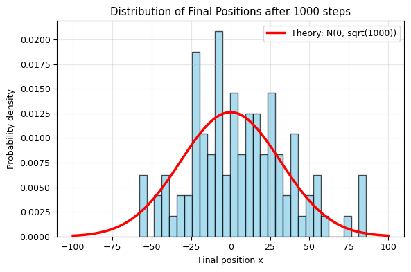
After N = 1000 steps:
<x^2> observed: 1013
<x^2> expected: 1000
<x>:          6.04 (should be approx 0)
std(x):       31.2 approx sqrt(1000) = 31.6
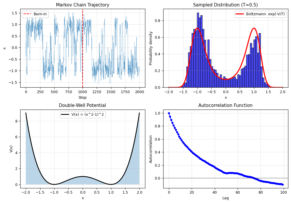
III. The Metropolis Algorithm#
Sampling from Complicated Distributions#
Problem: We want to sample from a distribution P(x) proportional to exp(-V(x)/T), but we can’t invert it.
Solution: Metropolis Algorithm
Propose a new state x_new = x + delta_x (random step)
Calculate acceptance probability: alpha = min(1, exp(-Delta_V/T)) where Delta_V = V(x_new) - V(x)
Accept/reject:
If rand() < alpha: accept x_new (move)
Else: stay at x
Repeat many times to build a chain
Why it works: The algorithm satisfies detailed balance, which ensures the stationary distribution is exactly P(x)!
def potential(x):
    return (x**2 - 1)**2

def metropolis_sampling(n_steps, step_size, temperature):
    np.random.seed(42)

    x = 0.0
    trajectory = [x]
    n_accept = 0

    for step in range(n_steps):
        x_new = x + np.random.normal(0, step_size)

        dV = potential(x_new) - potential(x)

        if dV < 0 or np.random.rand() < np.exp(-dV / temperature):
            x = x_new
            n_accept += 1

        trajectory.append(x)

    acceptance_rate = n_accept / n_steps
    return np.array(trajectory), acceptance_rate

T = 0.5
step_size = 0.5
n_steps = 5000

trajectory, acc_rate = metropolis_sampling(n_steps, step_size, T)

print(f"Metropolis Sampling from Double-Well Potential")
print(f"Temperature T = {T}")
print(f"Step size = {step_size}")
print(f"Acceptance rate: {acc_rate:.1%}")
print(f"\nMarkov chain statistics:")
print(f"Mean position: {np.mean(trajectory[1000:]):.3f}")
print(f"Std deviation: {np.std(trajectory[1000:]):.3f}")
Metropolis Sampling from Double-Well Potential
Temperature T = 0.5
Step size = 0.5
Acceptance rate: 60.4%

Markov chain statistics:
Mean position: -0.185
Std deviation: 0.897
burn_in = 1000
samples = trajectory[burn_in:]

def autocorrelation(signal, max_lag=100):
    c = np.correlate(signal - np.mean(signal), signal - np.mean(signal), mode='full')
    c = c[len(c)//2:]
    return c / c[0]

fig, axes = plt.subplots(2, 2, figsize=(10, 7))

axes[0, 0].plot(trajectory[:2000], linewidth=0.5, alpha=0.7)
axes[0, 0].axvline(burn_in, color='r', linestyle='--', label='Burn-in')
axes[0, 0].set_xlabel('Step')
axes[0, 0].set_ylabel('x')
axes[0, 0].set_title('Markov Chain Trajectory')
axes[0, 0].legend()
axes[0, 0].grid(alpha=0.3)

axes[0, 1].hist(samples, bins=50, density=True, alpha=0.7, color='blue', edgecolor='black')

x_range = np.linspace(-2, 2, 200)
V_range = potential(x_range)
P_exact = np.exp(-V_range / T)
P_exact = P_exact / np.trapz(P_exact, x_range)
axes[0, 1].plot(x_range, P_exact, 'r-', lw=2.5, label='Boltzmann: exp(-V/T)')
axes[0, 1].set_xlabel('x')
axes[0, 1].set_ylabel('Probability density')
axes[0, 1].set_title(f'Sampled Distribution (T={T})')
axes[0, 1].legend()
axes[0, 1].grid(alpha=0.3)

axes[1, 0].plot(x_range, V_range, 'k-', lw=2, label='V(x) = (x^2-1)^2')
axes[1, 0].fill_between(x_range, V_range, alpha=0.3)
axes[1, 0].set_xlabel('x')
axes[1, 0].set_ylabel('V(x)')
axes[1, 0].set_title('Double-Well Potential')
axes[1, 0].legend()
axes[1, 0].grid(alpha=0.3)

acf = autocorrelation(samples, max_lag=100)
axes[1, 1].plot(acf[:100], 'bo-', ms=4)
axes[1, 1].axhline(0, color='k', linestyle='-', alpha=0.3)
axes[1, 1].set_xlabel('Lag')
axes[1, 1].set_ylabel('Autocorrelation')
axes[1, 1].set_title('Autocorrelation Function')
axes[1, 1].grid(alpha=0.3)

plt.tight_layout()
plt.show()
/tmp/ipykernel_828/272206957.py:24: DeprecationWarning: `trapz` is deprecated. Use `trapezoid` instead, or one of the numerical integration functions in `scipy.integrate`.
  P_exact = P_exact / np.trapz(P_exact, x_range)
III. Application: The 2D Ising Model (Phase Transition!)#
The Ising Model: Spins on a Lattice#
System: Spins s_i = +/-1 on a 2D square lattice
Energy: E = -J Σ sᵢsⱼ over nearest neighbors
J > 0: Ferromagnetic (spins want to align)
Each aligned pair contributes minus J (lower energy)
Temperature effects:
T to 0: System is ordered (all spins aligned)
T to infinity: System is random (thermal fluctuations dominate)
T_c ≈ 2.269 J/k_B: Critical temperature (phase transition!)
Magnetization: M = |sum s_i| / N
M ≈ 1 at low T (ordered)
M ≈ 0 at high T (disordered)
def ising_metropolis_step(spins, J, T):
    L = len(spins)
    n_accept = 0

    for i in range(L):
        for j in range(L):
            s_old = spins[i, j]

            neighbors = (spins[(i-1) % L, j] + spins[(i+1) % L, j] +
                        spins[i, (j-1) % L] + spins[i, (j+1) % L])
            dE = 2 * J * s_old * neighbors

            if dE < 0 or np.random.rand() < np.exp(-dE / T):
                spins[i, j] = -s_old
                n_accept += 1

    return n_accept

def run_ising(L, T, n_sweeps):
    J = 1.0

    spins = np.random.choice([-1, 1], size=(L, L))

    magnetization = []
    energy = []

    for sweep in range(n_sweeps):
        ising_metropolis_step(spins, J, T)

        M = np.abs(np.sum(spins)) / (L**2)
        E = 0
        for i in range(L):
            for j in range(L):
                neighbors = (spins[(i-1) % L, j] + spins[(i+1) % L, j] +
                            spins[i, (j-1) % L] + spins[i, (j+1) % L])
                E -= J * spins[i, j] * neighbors / 2
        E = E / (L**2)

        magnetization.append(M)
        energy.append(E)

    return spins, np.array(magnetization), np.array(energy)

print("Ising model functions defined. Ready to simulate!")
Ising model functions defined. Ready to simulate!
np.random.seed(42)

L = 20
n_sweeps = 500

temperatures = [0.5, 1.5, 2.269, 3.0, 5.0]
results = {}

print(f"Running Ising model on {L}x{L} lattice...\n")

for T in temperatures:
    spins, mag, eng = run_ising(L, T, n_sweeps)
    results[T] = {
        'spins': spins,
        'magnetization': mag,
        'energy': eng
    }

    m_avg = np.mean(mag[100:])
    e_avg = np.mean(eng[100:])
    print(f"T = {T:5.3f}:  <M> = {m_avg:.3f},  <E> = {e_avg:.4f}")
Running Ising model on 20x20 lattice...

T = 0.500:  <M> = 1.000,  <E> = -2.0000
T = 1.500:  <M> = 0.987,  <E> = -1.9523
T = 2.269:  <M> = 0.669,  <E> = -1.4376
T = 3.000:  <M> = 0.148,  <E> = -0.8253
T = 5.000:  <M> = 0.066,  <E> = -0.4269
fig, axes = plt.subplots(1, 3, figsize=(10, 3))
temps_to_plot = [0.5, 2.269, 5.0]
for idx, T in enumerate(temps_to_plot):
spins = results[T]['spins']
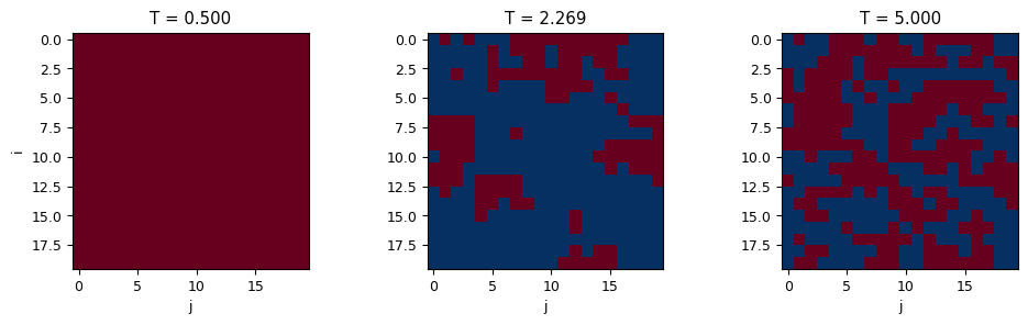
axes[idx].imshow(spins, cmap='RdBu', vmin=-1, vmax=1)
axes[idx].set_title(f'T = {T:.3f}')
axes[idx].set_xlabel('j')
if idx == 0:
axes[idx].set_ylabel('i')
else:
axes[idx].set_ylabel('')
plt.tight_layout()
plt.show()
print("\nSpin configurations:")
print(" T = 0.5: ORDERED (below Tc) - spins mostly aligned")
print(" T = 2.269: CRITICAL (at Tc) - domains of mixed sizes")
print(" T = 5.0: DISORDERED (above Tc) - random spins")
Spin configurations:
  T = 0.5:    ORDERED (below Tc) - spins mostly aligned
  T = 2.269:  CRITICAL (at Tc) - domains of mixed sizes
  T = 5.0:    DISORDERED (above Tc) - random spins
T_range = np.linspace(0.5, 6.0, 12)
magnetization_avg = []
energy_avg = []
print(f"Scanning temperature from {T_range[0]:.1f} to {T_range[-1]:.1f}...\n")
for T in T_range:
spins, mag, eng = run_ising(L, T, n_sweeps=300)
m_avg = np.mean(mag[100:])
e_avg = np.mean(eng[100:])
magnetization_avg.append(m_avg)
energy_avg.append(e_avg)
fig, axes = plt.subplots(1, 2, figsize=(10, 4))
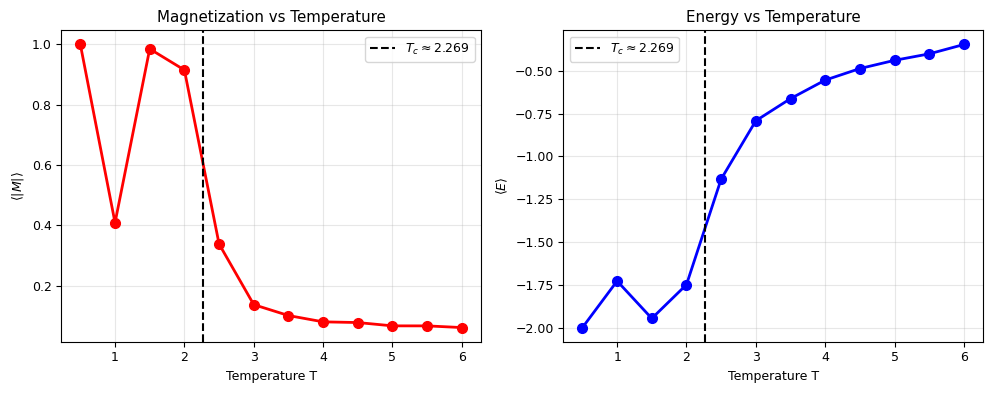
axes[0].plot(T_range, magnetization_avg, 'o-', color='red', ms=7, lw=2)
axes[0].axvline(2.269, color='k', linestyle='--', lw=1.5, label='$T_c \\approx 2.269$')
axes[0].set_xlabel('Temperature T')
axes[0].set_ylabel('$\\langle |M| \\rangle$')
axes[0].set_title('Magnetization vs Temperature')
axes[0].legend()
axes[0].grid(alpha=0.3)
axes[1].plot(T_range, energy_avg, 'o-', color='blue', ms=7, lw=2)
axes[1].axvline(2.269, color='k', linestyle='--', lw=1.5, label='$T_c \\approx 2.269$')
axes[1].set_xlabel('Temperature T')
axes[1].set_ylabel('$\\langle E \\rangle$')
axes[1].set_title('Energy vs Temperature')
axes[1].legend()
axes[1].grid(alpha=0.3)
plt.tight_layout()
plt.show()
print(f"\nPhase transition occurs at Tc ≈ 2.269 J/kB")
print(f"Below Tc: Ferromagnetic phase (M > 0)")
print(f"Above Tc: Paramagnetic phase (M ≈ 0)")
Scanning temperature from 0.5 to 6.0...
Phase transition occurs at Tc ≈ 2.269 J/kB
Below Tc: Ferromagnetic phase (M > 0)
Above Tc: Paramagnetic phase (M ≈ 0)