Lecture 13: Stochastic Methods II — Monte Carlo Integration#
Computational Physics — Spring 2026
From Random Numbers to Powerful Integrals#
In the previous lecture, we learned how to generate random numbers and use them for random walks, Metropolis sampling, and the Ising model. Today we turn randomness into a computational tool for integration.
The key insight: in high dimensions, deterministic quadrature (trapezoidal, Simpson’s, Gaussian) becomes hopelessly expensive — the number of grid points scales as \(N^d\). Monte Carlo integration sidesteps this curse of dimensionality because its error scales as \(1/\sqrt{N}\) regardless of dimension.
Today’s roadmap:
Monte Carlo integration and its error analysis
Importance sampling to reduce variance
Rejection sampling to generate arbitrary distributions
Application: Variational Monte Carlo for the hydrogen atom
The classic π estimation as a geometric MC example
import numpy as np
import matplotlib.pyplot as plt
from scipy import stats, integrate

plt.rcParams['figure.figsize'] = [6, 4]
plt.rcParams['font.size'] = 9

print("Ready for Monte Carlo integration!")
Ready for Monte Carlo integration!
I. Monte Carlo Integration#
The Basic Idea#
To compute the integral \(I = \int_a^b f(x)\, dx\), we can rewrite it as an expectation value:
where \(x_i\) are drawn uniformly from \([a, b]\).
Proof: Error Scales as \(1/\sqrt{N}\)#
Define the sample mean \(\bar{f}_N = \frac{1}{N}\sum_{i=1}^N f(x_i)\). Each \(f(x_i)\) is an i.i.d. random variable with:
Mean: \(\mu = \langle f \rangle = \frac{1}{b-a}\int_a^b f(x)\,dx\)
Variance: \(\sigma^2 = \langle f^2 \rangle - \langle f \rangle^2\)
By the Central Limit Theorem, the sample mean \(\bar{f}_N\) is approximately normal:
Therefore the standard error of the MC estimate is:
Key consequence: To halve the error, we need 4× more samples. This scaling is independent of dimension \(d\), which is the great advantage of MC over deterministic quadrature.
Method |
Error scaling (1D) |
Error scaling (\(d\)-D) |
|---|---|---|
Trapezoidal |
\(O(N^{-2})\) |
\(O(N^{-2/d})\) |
Simpson’s |
\(O(N^{-4})\) |
\(O(N^{-4/d})\) |
Monte Carlo |
\(O(N^{-1/2})\) |
\(O(N^{-1/2})\) |
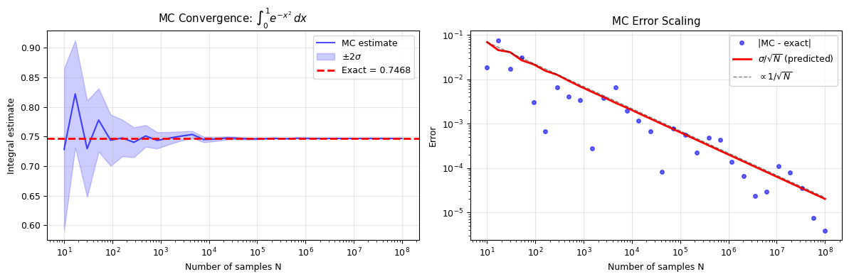
1D Example: \(\int_0^1 e^{-x^2}\,dx\)#
The exact value is \(\frac{\sqrt{\pi}}{2}\,\text{erf}(1) \approx 0.7468\). Let’s compute it with MC and verify the \(1/\sqrt{N}\) error scaling.
from scipy.special import erf

exact = np.sqrt(np.pi) / 2 * erf(1)
print(f"Exact value: {exact:.10f}")

np.random.seed(42)

# MC integration for various N
N_values = np.logspace(1, 8, 30, dtype=int)
N_values = np.unique(N_values)
mc_estimates = []
mc_errors = []

for N in N_values:
    x = np.random.uniform(0, 1, N)
    f_x = np.exp(-x**2)

    # sum(f_x) / N
    # MC estimate: (b-a) * mean(f)
    I_mc = np.mean(f_x)  # b-a = 1

    # Estimated standard error
    sigma = np.std(f_x, ddof=1)
    error = sigma / np.sqrt(N)

    mc_estimates.append(I_mc)
    mc_errors.append(error)

mc_estimates = np.array(mc_estimates)
mc_errors = np.array(mc_errors)

# Verify convergence
print(f"\nN = {N_values[-1]:>7d}:  MC = {mc_estimates[-1]:.6f},  error = {mc_errors[-1]:.2e}")
print(f"Absolute error: {abs(mc_estimates[-1] - exact):.2e}")
Exact value: 0.7468241328

N = 100000000:  MC = 0.746828,  error = 2.01e-05
Absolute error: 3.90e-06
fig, axes = plt.subplots(1, 2, figsize=(12, 4))

# Left: MC estimate vs N
axes[0].semilogx(N_values, mc_estimates, 'b-', alpha=0.7, label='MC estimate')
axes[0].fill_between(N_values, mc_estimates - 2*mc_errors, mc_estimates + 2*mc_errors,
                     alpha=0.2, color='blue', label='$\\pm 2\\sigma$')
axes[0].axhline(exact, color='r', linestyle='--', lw=2, label=f'Exact = {exact:.4f}')
axes[0].set_xlabel('Number of samples N')
axes[0].set_ylabel('Integral estimate')
axes[0].set_title('MC Convergence: $\\int_0^1 e^{-x^2}\\,dx$')
axes[0].legend()
axes[0].grid(alpha=0.3)

# Right: Error vs N (log-log)
actual_errors = np.abs(mc_estimates - exact)
axes[1].loglog(N_values, actual_errors, 'bo', ms=4, alpha=0.6, label='|MC - exact|')
axes[1].loglog(N_values, mc_errors, 'r-', lw=2, label='$\\sigma/\\sqrt{N}$ (predicted)')

# Reference 1/sqrt(N) line
C = mc_errors[0] * np.sqrt(N_values[0])
axes[1].loglog(N_values, C / np.sqrt(N_values), 'k--', lw=1, alpha=0.5, label='$\\propto 1/\\sqrt{N}$')

axes[1].set_xlabel('Number of samples N')
axes[1].set_ylabel('Error')
axes[1].set_title('MC Error Scaling')
axes[1].legend()
axes[1].grid(alpha=0.3)

plt.tight_layout()
plt.show()

print("Error follows 1/sqrt(N) — confirmed!")
Error follows 1/sqrt(N) — confirmed!
The Curse of Dimensionality: Volume of a Hypersphere#
The volume of a unit hypersphere in \(d\) dimensions is:
We can estimate this with MC by sampling uniformly in the \([-1, 1]^d\) hypercube and counting the fraction of points inside the unit sphere (\(\sum x_i^2 \leq 1\)):
This works in any dimension with the same \(1/\sqrt{N}\) scaling!
from scipy.special import gamma

def hypersphere_volume_exact(d):
    """Exact volume of unit hypersphere in d dimensions."""
    return np.pi**(d/2) / gamma(d/2 + 1)

def hypersphere_volume_mc(d, N):
    """MC estimate of hypersphere volume by sampling in [-1,1]^d cube."""
    points = np.random.uniform(-1, 1, size=(N, d))
    r_squared = np.sum(points**2, axis=1)
    n_inside = np.sum(r_squared <= 1)

    volume = (2**d) * n_inside / N
    # Binomial standard error
    p = n_inside / N
    error = (2**d) * np.sqrt(p * (1 - p) / N)
    return volume, error

np.random.seed(42)
N = 1000000

print(f"Volume of unit hypersphere (N = {N:,} samples)\n")
print(f"{'d':>3s}  {'V_exact':>12s}  {'V_MC':>12s}  {'Error':>10s}  {'Rel.Err':>10s}  {'Fraction inside':>16s}")
print("-" * 75)

for d in [2, 3, 5, 8, 10, 15, 20]:
    V_exact = hypersphere_volume_exact(d)
    V_mc, err = hypersphere_volume_mc(d, N)
    frac = V_mc / (2**d)
    rel_err = abs(V_mc - V_exact) / V_exact if V_exact > 0 else float('inf')
    print(f"{d:3d}  {V_exact:12.6f}  {V_mc:12.6f}  {err:10.4f}  {rel_err:10.2%}  {frac:16.6f}")
Volume of unit hypersphere (N = 1,000,000 samples)

  d       V_exact          V_MC       Error     Rel.Err   Fraction inside
---------------------------------------------------------------------------
  2      3.141593      3.141952      0.0016       0.01%          0.785488
  3      4.188790      4.189088      0.0040       0.01%          0.523636
  5      5.263789      5.246048      0.0118       0.34%          0.163939
  8      4.058712      4.049664      0.0319       0.22%          0.015819
 10      2.550164      2.553856      0.0511       0.14%          0.002494
 15      0.381443      0.524288      0.1311      37.45%          0.000016
 20      0.025807      0.000000      0.0000     100.00%          0.000000
# Visualize: hypersphere volume shrinks rapidly with dimension
dims = np.arange(1, 25)
volumes_exact = [hypersphere_volume_exact(d) for d in dims]

fig, ax = plt.subplots(figsize=(8, 4))
ax.semilogy(dims, volumes_exact, 'ro-', ms=6, lw=2)
ax.set_xlabel('Dimension d')
ax.set_ylabel('Volume of unit hypersphere')
ax.set_title('The Curse of Dimensionality: Hypersphere Volume vs Dimension')
ax.grid(alpha=0.3)
ax.set_xticks(dims[::2])
plt.tight_layout()
plt.show()

print(f"\nIn d=2: V = {hypersphere_volume_exact(2):.4f} (= π)")
print(f"In d=3: V = {hypersphere_volume_exact(3):.4f} (= 4π/3)")
print(f"In d=10: V = {hypersphere_volume_exact(10):.4f}")
print(f"In d=20: V = {hypersphere_volume_exact(20):.2e}")
print(f"\nThe sphere occupies a vanishingly small fraction of the cube in high dimensions.")
print(f"This is why high-dimensional integration is hard — most of the volume is in the corners!")
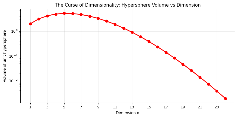
In d=2: V = 3.1416 (= π)
In d=3: V = 4.1888 (= 4π/3)
In d=10: V = 2.5502
In d=20: V = 2.58e-02

The sphere occupies a vanishingly small fraction of the cube in high dimensions.
This is why high-dimensional integration is hard — most of the volume is in the corners!
II. Importance Sampling#
The Problem with Uniform Sampling#
Basic MC samples uniformly, but if \(f(x)\) is sharply peaked, most samples contribute almost nothing to the integral. We waste computational effort sampling where \(f(x) \approx 0\).
The Solution: Sample Where It Matters#
Key identity: For any probability density \(g(x) > 0\) on \([a, b]\):
If we draw samples \(x_i \sim g(x)\) instead of uniformly, the MC estimate becomes:
Proof: Optimal Importance Sampling Distribution#
The variance of the importance-sampled estimator is:
To minimize this, we use the calculus of variations (or Cauchy-Schwarz). The result is:
i.e., the optimal sampling distribution is proportional to \(|f(x)|\) itself! With \(g = g^*\), the variance is exactly zero — but this requires knowing \(\int |f|\) in advance, which is the integral we’re trying to compute.
In practice, we choose \(g(x)\) to approximate the shape of \(|f(x)|\) using a known, easy-to-sample distribution.
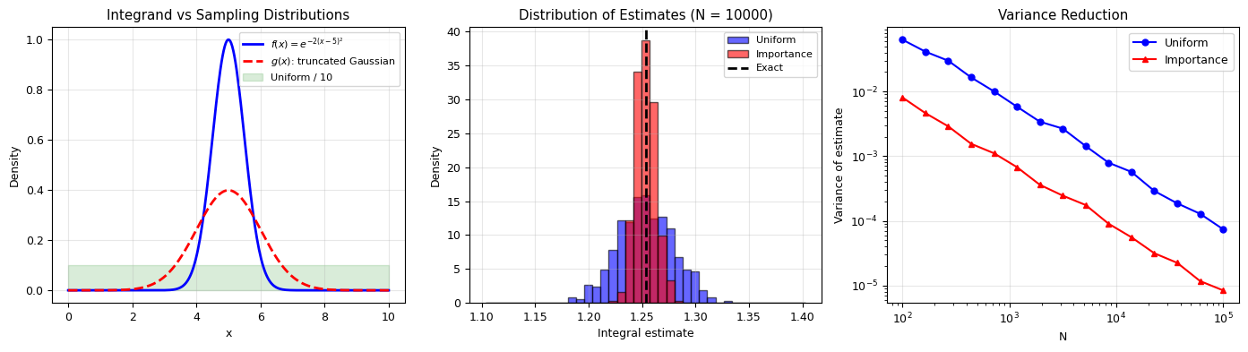
Demo: Integrating a Sharply Peaked Function#
Consider: $\(I = \int_0^{10} e^{-2(x-5)^2}\,dx\)$
This is sharply peaked around \(x = 5\). Uniform sampling on \([0, 10]\) wastes most samples in the tails.
def f_peaked(x):
    """Sharply peaked function."""
    return np.exp(-2 * (x - 5)**2)

# Exact value via scipy
exact_peaked, _ = integrate.quad(f_peaked, 0, 10)
print(f"Exact integral: {exact_peaked:.10f}")

np.random.seed(42)
N = 10000
n_trials = 500  # Repeat to measure variance

# Method 1: Uniform sampling
uniform_estimates = []
for _ in range(n_trials):
    x = np.random.uniform(0, 10, N)
    I_uniform = 10 * np.mean(f_peaked(x))  # (b-a) * mean(f)
    uniform_estimates.append(I_uniform)

# Method 2: Importance sampling with g(x) = Normal(5, 1) truncated to [0,10]
# g(x) = phi((x-5)/1) / (Phi(5) - Phi(-5))  on [0,10]
from scipy.stats import truncnorm

a_trunc, b_trunc = (0 - 5) / 1.0, (10 - 5) / 1.0  # standardized bounds
g_dist = truncnorm(a_trunc, b_trunc, loc=5, scale=1)

importance_estimates = []
for _ in range(n_trials):
    x = g_dist.rvs(N)
    weights = f_peaked(x) / g_dist.pdf(x)
    I_importance = np.mean(weights)
    importance_estimates.append(I_importance)

uniform_estimates = np.array(uniform_estimates)
importance_estimates = np.array(importance_estimates)

print(f"\nUniform sampling (N = {N}):")
print(f"  Mean:    {np.mean(uniform_estimates):.6f}")
print(f"  Std dev: {np.std(uniform_estimates):.6f}")

print(f"\nImportance sampling (N = {N}, g = truncated Gaussian):")
print(f"  Mean:    {np.mean(importance_estimates):.6f}")
print(f"  Std dev: {np.std(importance_estimates):.6f}")

variance_ratio = np.var(uniform_estimates) / np.var(importance_estimates)
print(f"\nVariance reduction factor: {variance_ratio:.1f}x")
Exact integral: 1.2533141373

Uniform sampling (N = 10000):
  Mean:    1.253168
  Std dev: 0.025724

Importance sampling (N = 10000, g = truncated Gaussian):
  Mean:    1.253185
  Std dev: 0.009374

Variance reduction factor: 7.5x
fig, axes = plt.subplots(1, 3, figsize=(14, 4))

# Left: the integrand and sampling distributions
x_plot = np.linspace(0, 10, 300)
axes[0].plot(x_plot, f_peaked(x_plot), 'b-', lw=2, label='$f(x) = e^{-2(x-5)^2}$')
axes[0].plot(x_plot, g_dist.pdf(x_plot), 'r--', lw=2, label='$g(x)$: truncated Gaussian')
axes[0].fill_between(x_plot, 0, 0.1, alpha=0.15, color='green', label='Uniform / 10')
axes[0].set_xlabel('x')
axes[0].set_ylabel('Density')
axes[0].set_title('Integrand vs Sampling Distributions')
axes[0].legend(fontsize=8)
axes[0].grid(alpha=0.3)

# Middle: histogram of estimates
bins = np.linspace(exact_peaked - 0.15, exact_peaked + 0.15, 40)
axes[1].hist(uniform_estimates, bins=bins, alpha=0.6, color='blue',
             edgecolor='black', label='Uniform', density=True)
axes[1].hist(importance_estimates, bins=bins, alpha=0.6, color='red',
             edgecolor='black', label='Importance', density=True)
axes[1].axvline(exact_peaked, color='k', linestyle='--', lw=2, label='Exact')
axes[1].set_xlabel('Integral estimate')
axes[1].set_ylabel('Density')
axes[1].set_title(f'Distribution of Estimates (N = {N})')
axes[1].legend(fontsize=8)
axes[1].grid(alpha=0.3)

# Right: variance reduction vs N
N_scan = np.logspace(2, 5, 15, dtype=int)
N_scan = np.unique(N_scan)
var_uniform = []
var_importance = []

for N_i in N_scan:
    u_est = []
    i_est = []
    for _ in range(200):
        x_u = np.random.uniform(0, 10, N_i)
        u_est.append(10 * np.mean(f_peaked(x_u)))

        x_i = g_dist.rvs(N_i)
        i_est.append(np.mean(f_peaked(x_i) / g_dist.pdf(x_i)))
    var_uniform.append(np.var(u_est))
    var_importance.append(np.var(i_est))

axes[2].loglog(N_scan, var_uniform, 'bo-', ms=5, label='Uniform')
axes[2].loglog(N_scan, var_importance, 'r^-', ms=5, label='Importance')
axes[2].set_xlabel('N')
axes[2].set_ylabel('Variance of estimate')
axes[2].set_title('Variance Reduction')
axes[2].legend()
axes[2].grid(alpha=0.3)

plt.tight_layout()
plt.show()
III. Rejection Sampling#
Generating Samples from Arbitrary Distributions#
Problem: We want to draw samples from a target distribution \(p(x)\), but we can’t invert its Cumulative Distribution Function (CDF).
Solution — Rejection Sampling:
Choose a proposal distribution \(q(x)\) that we can sample from
Find a constant \(M\) such that \(M \cdot q(x) \geq p(x)\) for all \(x\) (an “envelope”)
Draw \(x \sim q(x)\) and \(u \sim \text{Uniform}(0, 1)\)
Accept \(x\) if \(u < \frac{p(x)}{M \cdot q(x)}\); otherwise reject and try again
Proof: Accepted Samples Follow \(p(x)\)#
The probability of accepting a sample at position \(x\) is:
The joint density of proposing \(x\) and accepting it is:
Since \(\int \frac{p(x)}{M} dx = \frac{1}{M}\), the normalized distribution of accepted samples is:
The overall acceptance rate is \(1/M\), so we want \(M\) as small as possible (tight envelope).
Geometric Interpretation#
Think of it as “throwing darts” at the region under \(M \cdot q(x)\). Points that land under \(p(x)\) are kept; points between \(p(x)\) and \(M \cdot q(x)\) are discarded. The efficiency equals the ratio of areas:
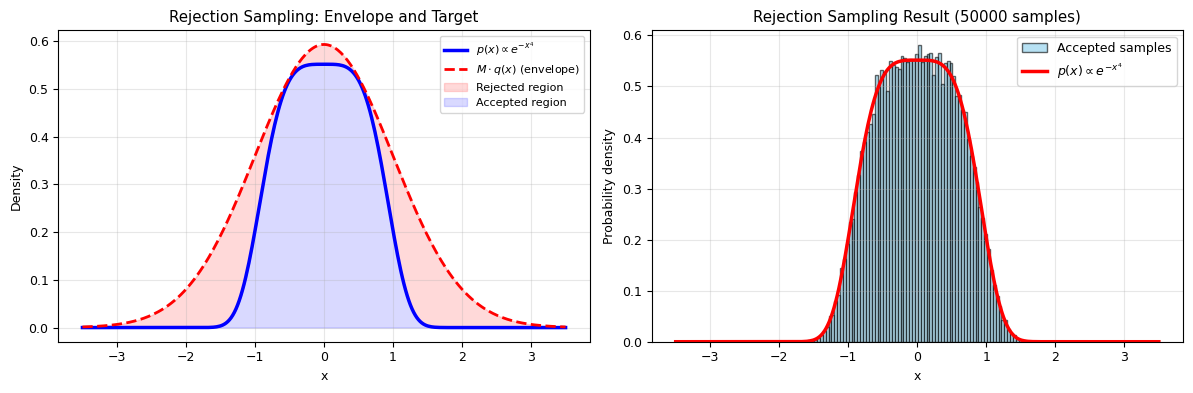
Demo: Sampling from \(p(x) \propto e^{-x^4}\)#
This “super-Gaussian” distribution has heavier tails than a Gaussian near the origin but thinner tails far out. There’s no closed-form CDF, so we use rejection sampling with a Gaussian proposal.
# Target distribution: p(x) proportional to exp(-x^4)
def p_unnorm(x):
    return np.exp(-x**4)

# Compute normalization constant numerically
Z, _ = integrate.quad(p_unnorm, -10, 10)
print(f"Normalization constant Z = {Z:.6f}")

def p_target(x):
    return p_unnorm(x) / Z

# Proposal: Gaussian with sigma chosen to envelope p(x)
# We need M such that M * q(x) >= p(x) for all x
sigma_q = 1.0
q_dist = stats.norm(0, sigma_q)

# Find M = max(p(x) / q(x))
x_grid = np.linspace(-4, 4, 10000)
ratio = p_target(x_grid) / q_dist.pdf(x_grid)
M = np.max(ratio) * 1.01  # small safety margin
print(f"Envelope constant M = {M:.4f}")
print(f"Expected acceptance rate: {1/M:.1%}")

# Rejection sampling
np.random.seed(42)
N_target = 50000
samples = []
n_proposed = 0

while len(samples) < N_target:
    x = q_dist.rvs()
    u = np.random.uniform()
    n_proposed += 1

    if u < p_target(x) / (M * q_dist.pdf(x)):
        samples.append(x)

samples = np.array(samples)
actual_rate = N_target / n_proposed

print(f"\nGenerated {N_target} samples from {n_proposed} proposals")
print(f"Actual acceptance rate: {actual_rate:.1%}")
print(f"Sample mean: {np.mean(samples):.4f} (expected: 0)")
print(f"Sample std:  {np.std(samples):.4f}")
Normalization constant Z = 1.812805
Envelope constant M = 1.4866
Expected acceptance rate: 67.3%

Generated 50000 samples from 74150 proposals
Actual acceptance rate: 67.4%
Sample mean: -0.0006 (expected: 0)
Sample std:  0.5794
fig, axes = plt.subplots(1, 2, figsize=(12, 4))

# Left: envelope visualization
x_plot = np.linspace(-3.5, 3.5, 300)
axes[0].plot(x_plot, p_target(x_plot), 'b-', lw=2.5, label='$p(x) \\propto e^{-x^4}$')
axes[0].plot(x_plot, M * q_dist.pdf(x_plot), 'r--', lw=2, label=f'$M \\cdot q(x)$ (envelope)')
axes[0].fill_between(x_plot, p_target(x_plot), M * q_dist.pdf(x_plot),
                     alpha=0.15, color='red', label='Rejected region')
axes[0].fill_between(x_plot, 0, p_target(x_plot),
                     alpha=0.15, color='blue', label='Accepted region')
axes[0].set_xlabel('x')
axes[0].set_ylabel('Density')
axes[0].set_title('Rejection Sampling: Envelope and Target')
axes[0].legend(fontsize=8)
axes[0].grid(alpha=0.3)

# Right: histogram of accepted samples vs target
axes[1].hist(samples, bins=80, density=True, alpha=0.6, color='skyblue',
             edgecolor='black', label='Accepted samples')
axes[1].plot(x_plot, p_target(x_plot), 'r-', lw=2.5, label='$p(x) \\propto e^{-x^4}$')
axes[1].set_xlabel('x')
axes[1].set_ylabel('Probability density')
axes[1].set_title(f'Rejection Sampling Result ({N_target} samples)')
axes[1].legend()
axes[1].grid(alpha=0.3)

plt.tight_layout()
plt.show()
IV. Application: Variational Monte Carlo for the Hydrogen Atom#
The Variational Principle#
For any trial wavefunction \(\psi_T(\mathbf{r}; \alpha)\) with variational parameter \(\alpha\), the variational principle guarantees:
where \(E_0\) is the true ground state energy. Minimizing \(E(\alpha)\) gives the best approximation within our trial function family.
Hydrogen Atom Setup#
The Hamiltonian (in atomic units: \(\hbar = m_e = e = 1\)):
Trial wavefunction: \(\psi_T(r; \alpha) = e^{-\alpha r}\)
The local energy is defined as:
For our trial wavefunction, applying \(\hat{H}\) in spherical coordinates:
The variational energy is then:
We evaluate this integral by sampling positions from \(|\psi_T|^2\) and averaging \(E_L\).
Analytical Result (for verification)#
For \(\psi_T = e^{-\alpha r}\), the exact variational energy is:
Minimizing: \(dE/d\alpha = \alpha - 1 = 0 \Rightarrow \alpha^* = 1\), giving \(E^* = -0.5\) Hartree \(= -13.6\) eV.
This is exact because \(e^{-r}\) is the true ground state wavefunction of hydrogen!
def local_energy(r, alpha):
    """Local energy for hydrogen atom with trial wavefunction exp(-alpha*r).
    E_L(r) = -alpha^2/2 + (alpha - 1)/r
    """
    return -alpha**2 / 2 + (alpha - 1) / r

def sample_hydrogen_wf(alpha, N):
    """Sample positions from |psi_T|^2 = exp(-2*alpha*r).

    The radial distribution is P(r) = 4*pi*r^2 * exp(-2*alpha*r) / (pi/alpha^3)
    which is a Gamma distribution in r.
    Specifically, 2*alpha*r follows Gamma(3, 1), so r = Gamma(3,1) / (2*alpha).
    """
    # r follows the distribution P(r) ∝ r^2 exp(-2αr)
    # This is a Gamma(3, scale=1/(2α)) distribution
    r = np.random.gamma(3, scale=1/(2*alpha), size=N)
    return r

def vmc_energy(alpha, N):
    """Compute variational energy E(alpha) via Monte Carlo."""
    r = sample_hydrogen_wf(alpha, N)
    E_L = local_energy(r, alpha)
    E_mean = np.mean(E_L)
    E_err = np.std(E_L) / np.sqrt(N)
    return E_mean, E_err

def analytical_energy(alpha):
    """Exact variational energy for exp(-alpha*r) trial wavefunction."""
    return alpha**2 / 2 - alpha

# Test at alpha = 1 (exact ground state)
np.random.seed(42)
E, err = vmc_energy(1.0, 10000)
print(f"VMC at alpha = 1.0:  E = {E:.6f} ± {err:.6f} Hartree")
print(f"Exact:               E = {analytical_energy(1.0):.6f} Hartree")
print(f"                       = {analytical_energy(1.0) * 27.2114:.2f} eV")
VMC at alpha = 1.0:  E = -0.500000 ± 0.000000 Hartree
Exact:               E = -0.500000 Hartree
                       = -13.61 eV
# Scan alpha to find the minimum
np.random.seed(42)
alphas = np.linspace(0.3, 2.0, 30)
E_mc = []
E_mc_err = []
E_exact = []

N_mc = 100000

for alpha in alphas:
    E, err = vmc_energy(alpha, N_mc)
    E_mc.append(E)
    E_mc_err.append(err)
    E_exact.append(analytical_energy(alpha))

E_mc = np.array(E_mc)
E_mc_err = np.array(E_mc_err)
E_exact = np.array(E_exact)

# Find VMC minimum
idx_min = np.argmin(E_mc)
alpha_min = alphas[idx_min]
E_min = E_mc[idx_min]

print(f"VMC minimum: alpha = {alpha_min:.3f}, E = {E_min:.6f} Hartree")
print(f"Exact minimum: alpha = 1.000, E = -0.500000 Hartree")
print(f"\nGround state energy: {E_min * 27.2114:.2f} eV (exact: -13.61 eV)")
VMC minimum: alpha = 1.003, E = -0.499991 Hartree
Exact minimum: alpha = 1.000, E = -0.500000 Hartree

Ground state energy: -13.61 eV (exact: -13.61 eV)
fig, axes = plt.subplots(1, 2, figsize=(12, 4))

# Left: E(alpha) curve
axes[0].errorbar(alphas, E_mc, yerr=2*E_mc_err, fmt='bo', ms=4, capsize=2,
                 label='VMC ($\\pm 2\\sigma$)', alpha=0.7)
axes[0].plot(alphas, E_exact, 'r-', lw=2, label='Exact: $\\alpha^2/2 - \\alpha$')
axes[0].axvline(1.0, color='k', linestyle=':', alpha=0.5)
axes[0].axhline(-0.5, color='k', linestyle=':', alpha=0.5)
axes[0].plot(1.0, -0.5, 'k*', ms=15, label='True ground state')
axes[0].set_xlabel('Variational parameter $\\alpha$')
axes[0].set_ylabel('Energy (Hartree)')
axes[0].set_title('Variational Monte Carlo: Hydrogen Atom')
axes[0].legend(fontsize=8)
axes[0].grid(alpha=0.3)

# Right: wavefunction and local energy at alpha=1
r_plot = np.linspace(0.01, 6, 300)
psi = np.exp(-r_plot)
psi_sq = psi**2
E_L_plot = local_energy(r_plot, 1.0)

ax2 = axes[1]
ax2.plot(r_plot, 4*np.pi*r_plot**2 * psi_sq / (np.pi), 'b-', lw=2,
         label='$4\\pi r^2 |\\psi|^2$ (radial probability)')
ax2.axhline(-0.5, color='r', linestyle='--', lw=2, label='$E_L = -0.5$ (constant!)')
ax2.set_xlabel('$r$ (Bohr radii)')
ax2.set_ylabel('Density / Energy')
ax2.set_title('Hydrogen Ground State ($\\alpha = 1$)')
ax2.legend(fontsize=8)
ax2.grid(alpha=0.3)
ax2.set_ylim(-1.5, 1.5)

plt.tight_layout()
plt.show()

print("At alpha = 1 (exact wavefunction), E_L(r) = -0.5 everywhere — zero variance!")
print("This is the 'zero-variance property': when psi_T = psi_exact, the local energy is constant.")
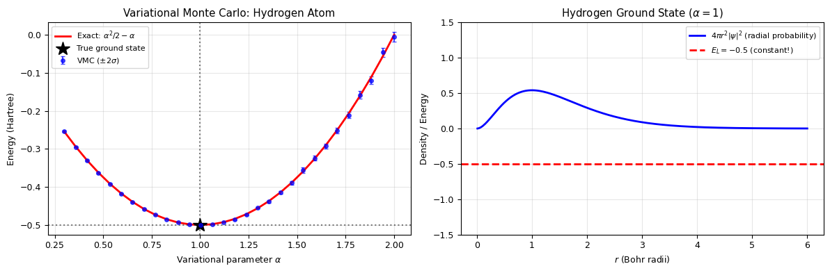
At alpha = 1 (exact wavefunction), E_L(r) = -0.5 everywhere — zero variance!
This is the 'zero-variance property': when psi_T = psi_exact, the local energy is constant.
# Show the zero-variance property: variance of E_L vs alpha
np.random.seed(42)
alphas_fine = np.linspace(0.5, 1.5, 25)
variances = []

for alpha in alphas_fine:
    r = sample_hydrogen_wf(alpha, 100000)
    E_L = local_energy(r, alpha)
    variances.append(np.var(E_L))

fig, ax = plt.subplots(figsize=(6, 4))
ax.plot(alphas_fine, variances, 'go-', ms=5, lw=2)
ax.axvline(1.0, color='r', linestyle='--', label='$\\alpha = 1$ (exact)')
ax.set_xlabel('Variational parameter $\\alpha$')
ax.set_ylabel('Var($E_L$)')
ax.set_title('Zero-Variance Property: Var($E_L$) → 0 as $\\psi_T$ → $\\psi_{exact}$')
ax.legend()
ax.grid(alpha=0.3)
plt.tight_layout()
plt.show()

print(f"Var(E_L) at alpha=1.0: {variances[len(variances)//2]:.2e}")
print(f"Var(E_L) at alpha=0.5: {variances[0]:.4f}")
print(f"Var(E_L) at alpha=1.5: {variances[-1]:.4f}")
print(f"\nThe variance vanishes at the exact wavefunction — this is a deep result!")
print(f"In practice, low variance of E_L indicates a good trial wavefunction.")
V. Estimating π: The Classic MC Example#
Dart-Throwing Method#
The simplest MC integration problem: throw random darts at a unit square \([0,1]^2\) and count the fraction that land inside the quarter-circle \(x^2 + y^2 \leq 1\).
Therefore: \(\pi \approx 4 \cdot \frac{N_{\text{inside}}}{N_{\text{total}}}\)
This is just MC integration of \(f(x,y) = \mathbf{1}[x^2 + y^2 \leq 1]\) over \([0,1]^2\).
np.random.seed(42)

N = 100000000
x = np.random.uniform(0, 1, N)
y = np.random.uniform(0, 1, N)

# finish the code to count points inside the quarter circle and estimate pi

# num_inside = 0
# for i in range(N):
#     xy = x[i]**2 + y[i]**2
#     if xy <=1:
#         num_inside += 1
# pi_estimate = num_inside / N * 4
# print (pi_estimate)

inside = x**2 + y**2 < 1
pi_estimate = np.sum(inside) / N * 4
print (pi_estimate)

# print(f"N = {N:,}")
print(f"Points inside quarter-circle: {np.sum(inside):,}")
print(f"π estimate: {pi_estimate:.6f}")
print(f"π exact:    {np.pi:.6f}")
print(f"Error:      {abs(pi_estimate - np.pi):.6f}")
3.14172304
Points inside quarter-circle: 78,543,076
π estimate: 3.141723
π exact:    3.141593
Error:      0.000130
fig, axes = plt.subplots(1, 2, figsize=(12, 5))

# Left: dart visualization (first 5000 points)
n_show = 5000
axes[0].scatter(x[:n_show][inside[:n_show]], y[:n_show][inside[:n_show]],
                s=1, c='blue', alpha=0.5, label='Inside')
axes[0].scatter(x[:n_show][~inside[:n_show]], y[:n_show][~inside[:n_show]],
                s=1, c='red', alpha=0.5, label='Outside')

theta = np.linspace(0, np.pi/2, 100)
axes[0].plot(np.cos(theta), np.sin(theta), 'k-', lw=2)
axes[0].set_xlim(0, 1)
axes[0].set_ylim(0, 1)
axes[0].set_aspect('equal')
axes[0].set_xlabel('x')
axes[0].set_ylabel('y')
axes[0].set_title(f'Dart Throwing ({n_show} points shown)')
axes[0].legend(markerscale=5)
axes[0].grid(alpha=0.3)

# Right: convergence of pi estimate
N_cum = np.arange(1, N+1)
pi_running = 4 * np.cumsum(inside) / N_cum

axes[1].semilogx(N_cum, pi_running, 'b-', lw=0.5, alpha=0.7)
axes[1].axhline(np.pi, color='r', linestyle='--', lw=2, label=f'$\\pi$ = {np.pi:.4f}')

# 1/sqrt(N) confidence band
p = np.pi / 4
sigma = 4 * np.sqrt(p * (1 - p))
N_plot = np.logspace(1, np.log10(N), 200)
axes[1].fill_between(N_plot,
                     np.pi - 2*sigma/np.sqrt(N_plot),
                     np.pi + 2*sigma/np.sqrt(N_plot),
                     alpha=0.2, color='red', label='$\\pm 2\\sigma/\\sqrt{N}$')

axes[1].set_xlabel('Number of darts N')
axes[1].set_ylabel('$\\pi$ estimate')
axes[1].set_title('Convergence of $\\pi$ Estimate')
axes[1].legend()
axes[1].grid(alpha=0.3)
axes[1].set_ylim(2.8, 3.5)

plt.tight_layout()
plt.show()

print(f"\nWith N = {N:,}: π ≈ {pi_estimate:.4f} (error = {abs(pi_estimate-np.pi):.4f})")
print(f"Predicted error (σ/√N): {sigma/np.sqrt(N):.4f}")
print(f"\nTo get 6 digits of π, we'd need N ~ (σ/10^{-6})^2 ≈ 10^{12} samples — MC is not efficient for π!")
print(f"But this same method works in 100 dimensions with the SAME error scaling.")
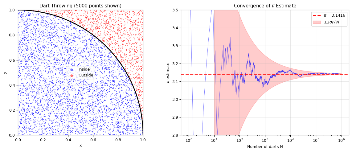
With N = 1,000,000: π ≈ 3.1419 (error = 0.0003)
Predicted error (σ/√N): 0.0016

To get 6 digits of π, we'd need N ~ (σ/10^-6)^2 ≈ 10^12 samples — MC is not efficient for π!
But this same method works in 100 dimensions with the SAME error scaling.