Lecture 09: The Fast Fourier Transform (FFT)#
Computational Physics — Spring 2026
Recap from Lecture 08#
We implemented the Discrete Fourier Transform (DFT) from scratch:
This required two nested loops → \(O(N^2)\) operations.
Today’s Goal#
The Fast Fourier Transform (FFT) computes the exact same DFT, but in \(O(N \log N)\) operations.
DFT (Lecture 08) |
FFT (Today) |
|
|---|---|---|
Result |
\(F_n\) |
Same \(F_n\) |
Complexity |
\(O(N^2)\) |
\(O(N \log N)\) |
N = 1024 |
~1,000,000 ops |
~10,000 ops |
N = 10⁶ |
~10¹² ops (~hours) |
~2×10⁷ ops (~seconds) |
The FFT is often called one of the most important algorithms of the 20th century (Cooley & Tukey, 1965).
import numpy as np
import matplotlib.pyplot as plt
from scipy import signal
import time

# Projector-friendly settings
plt.rcParams['figure.figsize'] = [6, 4]
plt.rcParams['font.size'] = 9

print("Ready!")
Ready!
I. Why Do We Need FFT?#
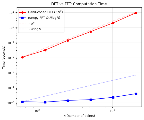
Our hand-coded DFT from Lecture 08 works, but it’s painfully slow for large \(N\).
Let’s measure it.
# Our hand-coded DFT from Lecture 08
def dft(f):
    """Compute the Discrete Fourier Transform (naive O(N^2) method).

    Parameters
    ----------
    f : array_like
        Input signal of length N.

    Returns
    -------
    F : ndarray
        DFT of the input signal.
    """
    N = len(f)
    F = np.zeros(N, dtype=complex)
    for n in range(N):
        for k in range(N):
            F[n] += f[k] * np.exp(-1j * 2 * np.pi * n * k / N)
    return F

# Timing comparison: DFT vs numpy FFT
N_values = [64, 128, 256, 512, 1024, 2048]
dft_times = []
fft_times = []

for N in N_values:
    x = np.random.randn(N)

    # Time our DFT
    t0 = time.time()
    F_dft = dft(x)
    dft_times.append(time.time() - t0)

    # Time numpy's FFT
    t0 = time.time()
    for _ in range(1000):  # Run 1000 times to get measurable time
        F_fft = np.fft.fft(x)
    fft_times.append((time.time() - t0) / 1000)

    # Verify they give the same answer!
    assert np.allclose(F_dft, F_fft), f"Mismatch at N={N}!"
    print(f"N={N:5d}:  DFT = {dft_times[-1]:.4f}s,  FFT = {fft_times[-1]:.6f}s,  "
          f"speedup = {dft_times[-1]/fft_times[-1]:.0f}x")
N=   64:  DFT = 0.0107s,  FFT = 0.000012s,  speedup = 903x
N=  128:  DFT = 0.0315s,  FFT = 0.000011s,  speedup = 2825x
N=  256:  DFT = 0.1410s,  FFT = 0.000014s,  speedup = 9755x
N=  512:  DFT = 0.5338s,  FFT = 0.000016s,  speedup = 32616x
N= 1024:  DFT = 2.0467s,  FFT = 0.000023s,  speedup = 87569x
N= 2048:  DFT = 9.5672s,  FFT = 0.000041s,  speedup = 235287x
# Plot timing comparison
fig, ax = plt.subplots(figsize=(6, 5))

ax.loglog(N_values, dft_times, 'ro-', label='Hand-coded DFT $O(N^2)$', markersize=6)
ax.loglog(N_values, fft_times, 'bs-', label='numpy FFT $O(N \log N)$', markersize=6)

# Theoretical scaling lines
N_arr = np.array(N_values, dtype=float)
ax.loglog(N_arr, dft_times[0] * (N_arr/N_arr[0])**2, 'r--', alpha=0.3, label='$\propto N^2$')
ax.loglog(N_arr, fft_times[0] * (N_arr*np.log2(N_arr))/(N_arr[0]*np.log2(N_arr[0])),
          'b--', alpha=0.3, label='$\propto N \log N$')

ax.set_xlabel('N (number of points)')
ax.set_ylabel('Time (seconds)')
ax.set_title('DFT vs FFT: Computation Time')
ax.legend()
ax.grid(True, alpha=0.3)
plt.tight_layout()
plt.show()
<>:5: SyntaxWarning: invalid escape sequence '\l'
<>:9: SyntaxWarning: invalid escape sequence '\p'
<>:11: SyntaxWarning: invalid escape sequence '\p'
<>:5: SyntaxWarning: invalid escape sequence '\l'
<>:9: SyntaxWarning: invalid escape sequence '\p'
<>:11: SyntaxWarning: invalid escape sequence '\p'
/tmp/ipython-input-654999808.py:5: SyntaxWarning: invalid escape sequence '\l'
  ax.loglog(N_values, fft_times, 'bs-', label='numpy FFT $O(N \log N)$', markersize=6)
/tmp/ipython-input-654999808.py:9: SyntaxWarning: invalid escape sequence '\p'
  ax.loglog(N_arr, dft_times[0] * (N_arr/N_arr[0])**2, 'r--', alpha=0.3, label='$\propto N^2$')
/tmp/ipython-input-654999808.py:11: SyntaxWarning: invalid escape sequence '\p'
  'b--', alpha=0.3, label='$\propto N \log N$')
The Speedup in Practice#
N |
DFT operations |
FFT operations |
Speedup |
|---|---|---|---|
10³ |
10⁶ |
10⁴ |
100× |
10⁴ |
10⁸ |
1.3×10⁵ |
750× |
10⁶ |
10¹² |
2×10⁷ |
50,000× |
10⁸ |
10¹⁶ |
2.7×10⁹ |
4,000,000× |
At \(N = 10^6\), the DFT would take hours. The FFT takes milliseconds.
This is not a different algorithm giving an approximation — it computes the exact same DFT, just smarter.
II. The Cooley-Tukey Algorithm#
The Key Idea: Divide and Conquer#
Split the sum into even-indexed and odd-indexed terms:
Separate even (\(k = 2m\)) and odd (\(k = 2m+1\)) terms:
Using \(W_N^{2} = W_{N/2}\):
where:
\(E_n = \text{DFT of even-indexed elements}\) (size \(N/2\))
\(O_n = \text{DFT of odd-indexed elements}\) (size \(N/2\))
\(W_N^n = e^{-2\pi i n/N}\) are called twiddle factors
The Symmetry Trick#
Since \(E_n\) and \(O_n\) have period \(N/2\):
This is the butterfly operation: one complex multiply + one add/subtract gives two output values!
Recursion: Keep Splitting!#
Each half-size DFT can be split again:
Number of levels: \(\log_2 N\)
Work per level: \(O(N)\) (butterfly operations)
Total: \(O(N \log N)\)
Requirement: \(N\) must be a power of 2 (for radix-2 FFT).
In practice, we zero-pad to the next power of 2.
def fft_recursive(x):
    """Compute FFT using the Cooley-Tukey radix-2 algorithm (recursive).

    Parameters
    ----------
    x : array_like
        Input signal. Length must be a power of 2.

    Returns
    -------
    F : ndarray
        FFT of the input signal.
    """
    N = len(x)

    # Base case: DFT of a single element is itself
    if N == 1:
        return np.array(x, dtype=complex)

    if N % 2 != 0:
        raise ValueError("Length must be a power of 2")

    # Recursively compute FFT of even and odd parts
    E = fft_recursive(x[0::2])   # Even-indexed: x[0], x[2], x[4], ...
    O = fft_recursive(x[1::2])   # Odd-indexed:  x[1], x[3], x[5], ...

    # Twiddle factors
    n = np.arange(N // 2)
    W = np.exp(-2j * np.pi * n / N)

    # Butterfly: combine even and odd
    F = np.zeros(N, dtype=complex)
    F[:N//2] = E + W * O       # First half
    F[N//2:] = E - W * O       # Second half (symmetry!)

    return F

# Test it!
x_test = np.random.randn(256)

F_ours = fft_recursive(x_test)
F_numpy = np.fft.fft(x_test)

print(f"Max difference: {np.max(np.abs(F_ours - F_numpy)):.2e}")
print(f"Match: {np.allclose(F_ours, F_numpy)}")
Max difference: 1.78e-14
Match: True
# Time our recursive FFT vs DFT vs numpy
N = 1024
x = np.random.randn(N)

t0 = time.time()
F1 = dft(x)
t_dft = time.time() - t0

t0 = time.time()
F2 = fft_recursive(x)
t_ours = time.time() - t0

t0 = time.time()
for _ in range(1000):
    F3 = np.fft.fft(x)
t_numpy = (time.time() - t0) / 1000

print(f"N = {N}")
print(f"Hand-coded DFT:    {t_dft:.4f} s")
print(f"Our recursive FFT: {t_ours:.4f} s  ({t_dft/t_ours:.1f}x faster than DFT)")
print(f"numpy FFT:         {t_numpy:.6f} s  ({t_dft/t_numpy:.0f}x faster than DFT)")
print(f"\nnumpy is {t_ours/t_numpy:.0f}x faster than our FFT")
print("(numpy uses optimized C code with FFTW-style algorithms)")
N = 1024
Hand-coded DFT:    2.0269 s
Our recursive FFT: 0.0106 s  (191.1x faster than DFT)
numpy FFT:         0.000038 s  (52911x faster than DFT)

numpy is 277x faster than our FFT
(numpy uses optimized C code with FFTW-style algorithms)
The Butterfly Diagram#
For N=8, the FFT computation flow looks like:
Input order:   x[0]  x[4]  x[2]  x[6]  x[1]  x[5]  x[3]  x[7]
               (bit-reversed order)

Stage 1:       ×---×  ×---×  ×---×  ×---×     (N/2 = 4 butterflies, size 2)
Stage 2:       ×---+--×     ×---+--×           (N/2 = 4 butterflies, size 4)
               ×---+--×     ×---+--×
Stage 3:       ×---+--+--+--×                  (N/2 = 4 butterflies, size 8)
               ×---+--+--+--×
               ×---+--+--+--×
               ×---+--+--+--×

Output:        F[0] F[1] F[2] F[3] F[4] F[5] F[6] F[7]
Each butterfly computes:
\(a + W \cdot b\) (top output)
\(a - W \cdot b\) (bottom output)
Total: \(\log_2(8) = 3\) stages × \(N/2 = 4\) butterflies = 12 complex multiplications
Compare: DFT needs \(N^2 = 64\) multiplications → 5× savings even at \(N=8\)!
III. Using numpy/scipy FFT in Practice#
Now that we understand how the FFT works, let’s use the optimized library functions.
Key Functions#
Function |
Purpose |
|---|---|
|
Forward FFT |
|
Inverse FFT |
|
Frequency axis (d = sample spacing) |
|
FFT for real signals (returns only positive frequencies) |
|
Shift zero-frequency to center |
|
2D FFT (for images) |
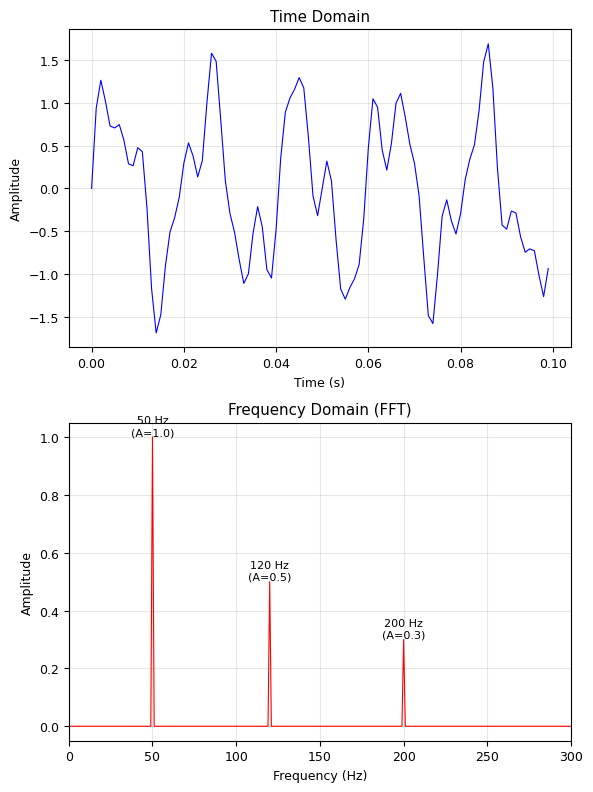
# Create a signal with known frequencies
fs = 1000          # Sampling rate (Hz)
T = 1.0            # Duration (s)
N = int(fs * T)    # Number of samples
t = np.linspace(0, T, N, endpoint=False)

# Signal: 50 Hz + 120 Hz + 200 Hz
x = 1.0 * np.sin(2 * np.pi * 50 * t) + \
    0.5 * np.sin(2 * np.pi * 120 * t) + \
    0.3 * np.sin(2 * np.pi * 200 * t)

# Compute FFT
F = np.fft.fft(x)
freqs = np.fft.fftfreq(N, d=1/fs)  # Frequency axis

# Plot
fig, (ax1, ax2) = plt.subplots(2, 1, figsize=(6, 8))

# Time domain
ax1.plot(t[:100], x[:100], 'b-', linewidth=0.8)
ax1.set_xlabel('Time (s)')
ax1.set_ylabel('Amplitude')
ax1.set_title('Time Domain')
ax1.grid(True, alpha=0.3)

# Frequency domain (only positive frequencies)
positive = freqs > 0
ax2.plot(freqs[positive],  2/N*np.abs(F[positive]), 'r-', linewidth=0.8)
ax2.set_xlabel('Frequency (Hz)')
ax2.set_ylabel('Amplitude')
ax2.set_title('Frequency Domain (FFT)')
ax2.set_xlim(0, 300)
ax2.grid(True, alpha=0.3)

# Annotate peaks
for freq, amp in [(50, 1.0), (120, 0.5), (200, 0.3)]:
    ax2.annotate(f'{freq} Hz\n(A={amp})', xy=(freq, amp), fontsize=8,
                ha='center', va='bottom')

plt.tight_layout()
plt.show()
# Understanding fftfreq
print("np.fft.fftfreq(N, d=1/fs) explained:")
print(f"  N = {N} samples")
print(f"  d = 1/fs = {1/fs} s (time between samples)")
print(f"  Frequency resolution: Δf = fs/N = {fs/N} Hz")
print(f"  Max frequency (Nyquist): fs/2 = {fs/2} Hz")
print()
print("First 10 frequencies:", freqs[:10])
print("Last 5 frequencies: ", freqs[-5:])
print("\nNote: negative frequencies appear in the second half!")
print("Use fftshift() to center them, or rfft() for real signals.")
np.fft.fftfreq(N, d=1/fs) explained:
  N = 1000 samples
  d = 1/fs = 0.001 s (time between samples)
  Frequency resolution: Δf = fs/N = 1.0 Hz
  Max frequency (Nyquist): fs/2 = 500.0 Hz

First 10 frequencies: [0. 1. 2. 3. 4. 5. 6. 7. 8. 9.]
Last 5 frequencies:  [-5. -4. -3. -2. -1.]

Note: negative frequencies appear in the second half!
Use fftshift() to center them, or rfft() for real signals.
# rfft: efficient FFT for real signals
# For real input, F[-n] = F[n]* (conjugate symmetry)
# So we only need the positive half!

F_full = np.fft.fft(x)       # Returns N complex values
F_real = np.fft.rfft(x)      # Returns N/2 + 1 complex values
freqs_real = np.fft.rfftfreq(N, d=1/fs)

print(f"fft output length:  {len(F_full)}")
print(f"rfft output length: {len(F_real)}  (about half!)")
print(f"\nFor real signals, rfft is ~2x faster and uses ~half the memory.")

# They give the same result for positive frequencies
print(f"Same result? {np.allclose(F_full[:N//2+1], F_real)}")
fft output length:  1000
rfft output length: 501  (about half!)

For real signals, rfft is ~2x faster and uses ~half the memory.
Same result? True
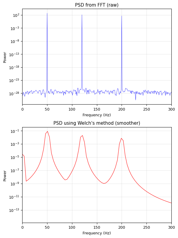
# Power Spectral Density (PSD)
# PSD = |F(f)|^2 / N — shows power at each frequency

# Method 1: Direct from FFT
psd_direct = (2 / N) * np.abs(F_real)**2

# Method 2: Welch's method (averages over segments, reduces noise)
freqs_welch, psd_welch = signal.welch(x, fs=fs, nperseg=256)

fig, (ax1, ax2) = plt.subplots(2, 1, figsize=(6, 8))

ax1.semilogy(freqs_real, psd_direct, 'b-', linewidth=0.5)
ax1.set_title('PSD from FFT (raw)')
ax1.set_xlabel('Frequency (Hz)')
ax1.set_ylabel('Power')
ax1.set_xlim(0, 300)
ax1.grid(True, alpha=0.3)

ax2.semilogy(freqs_welch, psd_welch, 'r-', linewidth=0.8)
ax2.set_title("PSD using Welch's method (smoother)")
ax2.set_xlabel('Frequency (Hz)')
ax2.set_ylabel('Power')
ax2.set_xlim(0, 300)
ax2.grid(True, alpha=0.3)

plt.tight_layout()
plt.show()
IV. Zero-Padding and Frequency Resolution#
Frequency Resolution#
To get finer frequency resolution, you need more data (larger \(N\) at the same \(f_s\)).
Zero-Padding#
Appending zeros to the signal before FFT interpolates the spectrum (smoother plot), but does NOT increase the true frequency resolution.
# Zero-padding demonstration
fs = 1000
N_orig = 64   # Short signal
t_orig = np.arange(N_orig) / fs
x_orig = np.sin(2 * np.pi * 50 * t_orig) + 0.7 * np.sin(2 * np.pi * 65 * t_orig)

# FFT without zero-padding
F1 = np.fft.rfft(x_orig)
f1 = np.fft.rfftfreq(N_orig, 1/fs)

# FFT with zero-padding to 256
N_pad = 256
x_padded = np.zeros(N_pad)
x_padded[:N_orig] = x_orig
F2 = np.fft.rfft(x_padded)
f2 = np.fft.rfftfreq(N_pad, 1/fs)

# FFT with zero-padding to 1024
N_pad2 = 1024
x_padded2 = np.zeros(N_pad2)
x_padded2[:N_orig] = x_orig
F3 = np.fft.rfft(x_padded2)
f3 = np.fft.rfftfreq(N_pad2, 1/fs)

fig, ax = plt.subplots(figsize=(6, 5))
ax.plot(f1, 2/N_orig * np.abs(F1), 'ro-', markersize=5, label=f'N={N_orig} (Δf={fs/N_orig:.1f} Hz)')
ax.plot(f2, 2/N_orig * np.abs(F2), 'b.-', markersize=3, label=f'Zero-padded to {N_pad}')
ax.plot(f3, 2/N_orig * np.abs(F3), 'g-', linewidth=0.8, label=f'Zero-padded to {N_pad2}')

ax.set_xlabel('Frequency (Hz)')
ax.set_ylabel('Amplitude')
ax.set_title('Zero-Padding: Interpolation, NOT Resolution')
ax.set_xlim(20, 100)
ax.legend(fontsize=7)
ax.grid(True, alpha=0.3)
plt.tight_layout()
plt.show()

print(f"Original Δf = {fs/N_orig:.1f} Hz — can barely resolve 50 and 65 Hz")
print(f"Zero-padding makes the plot smoother but doesn't separate the peaks better.")
print(f"To truly resolve two frequencies, you need: Δf < |f2 - f1| = 15 Hz")
print(f"→ Need N > fs/15 = {fs/15:.0f} samples of REAL data.")
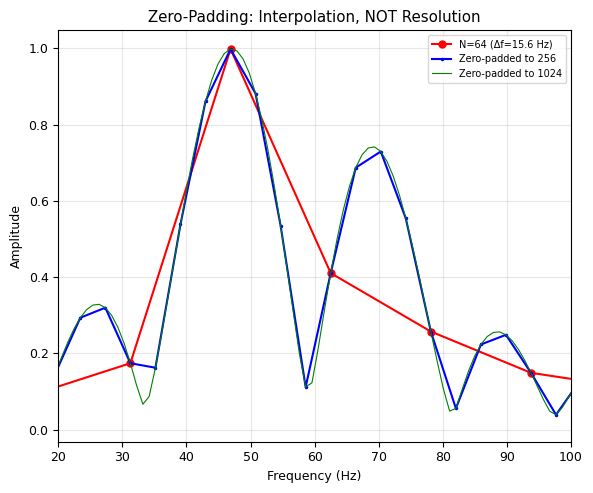
Original Δf = 15.6 Hz — can barely resolve 50 and 65 Hz
Zero-padding makes the plot smoother but doesn't separate the peaks better.
To truly resolve two frequencies, you need: Δf < |f2 - f1| = 15 Hz
→ Need N > fs/15 = 67 samples of REAL data.
V. Filtering in the Frequency Domain#
One of the most powerful applications of FFT:
FFT the signal → frequency domain
Modify the spectrum (zero out unwanted frequencies)
IFFT back → clean signal
This is \(O(N \log N)\) — much faster than convolution in the time domain!
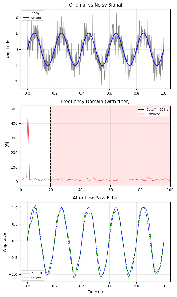
# Low-pass filter: remove high-frequency noise
fs = 1000
N = 1000
t = np.linspace(0, 1, N, endpoint=False)

# Clean signal: 5 Hz sine wave
x_clean = np.sin(2 * np.pi * 5 * t)

# Add high-frequency noise
np.random.seed(42)
x_noisy = x_clean + 0.5 * np.random.randn(N)

# FFT
F = np.fft.rfft(x_noisy)
freqs = np.fft.rfftfreq(N, d=1/fs)

# Low-pass filter: zero out everything above 20 Hz
cutoff = 20  # Hz
F_filtered = F.copy()
F_filtered[freqs > cutoff] = 0

# IFFT back to time domain
x_filtered = np.fft.irfft(F_filtered, n=N)

# Plot
fig, axes = plt.subplots(3, 1, figsize=(6, 10))

axes[0].plot(t, x_noisy, 'gray', linewidth=0.5, label='Noisy')
axes[0].plot(t, x_clean, 'b-', linewidth=1.5, label='Original')
axes[0].set_title('Original vs Noisy Signal')
axes[0].legend(fontsize=7)
axes[0].set_ylabel('Amplitude')
axes[0].grid(True, alpha=0.3)

axes[1].plot(freqs, np.abs(F), 'r-', linewidth=0.5)
axes[1].axvline(cutoff, color='k', linestyle='--', label=f'Cutoff = {cutoff} Hz')
axes[1].axvspan(cutoff, freqs[-1], alpha=0.1, color='red', label='Removed')
axes[1].set_title('Frequency Domain (with filter)')
axes[1].set_xlim(0, 100)
axes[1].set_ylabel('|F(f)|')
axes[1].legend(fontsize=7)
axes[1].grid(True, alpha=0.3)

axes[2].plot(t, x_filtered, 'g-', linewidth=1, label='Filtered')
axes[2].plot(t, x_clean, 'b--', linewidth=1, label='Original')
axes[2].set_title('After Low-Pass Filter')
axes[2].set_xlabel('Time (s)')
axes[2].set_ylabel('Amplitude')
axes[2].legend(fontsize=7)
axes[2].grid(True, alpha=0.3)

plt.tight_layout()
plt.show()
# Band-pass filter: extract a specific frequency range
# Simulated "ECG" signal with heart rate + noise + powerline interference
fs = 500
N = 5000
t = np.linspace(0, N/fs, N, endpoint=False)

# Heart signal: ~1.2 Hz (72 BPM) with harmonics
heart = (np.sin(2 * np.pi * 1.2 * t) +
         0.5 * np.sin(2 * np.pi * 2.4 * t) +
         0.3 * np.sin(2 * np.pi * 3.6 * t))

# Powerline interference at 60 Hz
powerline = 0.8 * np.sin(2 * np.pi * 60 * t)

# Random noise
np.random.seed(42)
noise = 0.3 * np.random.randn(N)

# Measured signal
ecg = heart + powerline + noise

# FFT and band-pass filter (keep 0.5 - 10 Hz)
F = np.fft.rfft(ecg)
freqs = np.fft.rfftfreq(N, d=1/fs)

# Band-pass: keep only 0.5 to 10 Hz
F_bp = F.copy()
F_bp[(freqs < 0.5) | (freqs > 10)] = 0

ecg_clean = np.fft.irfft(F_bp, n=N)

fig, axes = plt.subplots(3, 1, figsize=(6, 10))

axes[0].plot(t[:2000], ecg[:2000], 'gray', linewidth=0.5)
axes[0].set_title('Raw "ECG" Signal (heart + 60Hz powerline + noise)')
axes[0].set_ylabel('Amplitude')
axes[0].grid(True, alpha=0.3)

axes[1].semilogy(freqs, np.abs(F), 'r-', linewidth=0.5)
axes[1].axvspan(0.5, 10, alpha=0.2, color='green', label='Passband (0.5-10 Hz)')
axes[1].set_xlim(0, 80)
axes[1].set_title('Spectrum — notice 60 Hz peak!')
axes[1].set_ylabel('|F(f)|')
axes[1].legend(fontsize=7)
axes[1].grid(True, alpha=0.3)

axes[2].plot(t[:2000], ecg_clean[:2000], 'g-', linewidth=1, label='Filtered')
axes[2].plot(t[:2000], heart[:2000], 'b--', linewidth=1, alpha=0.5, label='True heart signal')
axes[2].set_title('After Band-Pass Filter (0.5–10 Hz)')
axes[2].set_xlabel('Time (s)')
axes[2].set_ylabel('Amplitude')
axes[2].legend(fontsize=7)
axes[2].grid(True, alpha=0.3)

plt.tight_layout()
plt.show()
print("60 Hz powerline interference completely removed!")
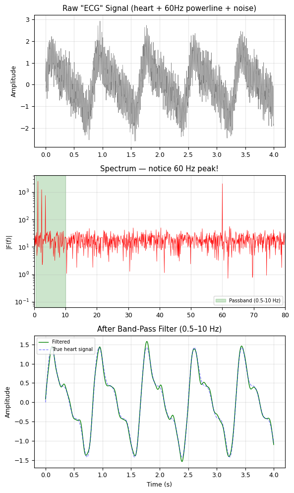
60 Hz powerline interference completely removed!
VI. 2D FFT and Image Processing#
Images are 2D signals. The 2D FFT decomposes an image into spatial frequencies:
Low spatial frequencies → smooth features, overall brightness
High spatial frequencies → edges, fine details, noise
# Create a test image: stripes + a circle
M, N_img = 256, 256
x = np.linspace(-1, 1, N_img)
y = np.linspace(-1, 1, M)
X, Y = np.meshgrid(x, y)

# Vertical stripes + horizontal stripes + gaussian blob
image = (np.sin(2 * np.pi * 8 * X) +         # Vertical stripes (8 cycles)
         0.5 * np.sin(2 * np.pi * 3 * Y) +    # Horizontal stripes (3 cycles)
         2 * np.exp(-(X**2 + Y**2) / 0.1))    # Gaussian blob

# 2D FFT
F_2d = np.fft.fft2(image)
F_shifted = np.fft.fftshift(F_2d)  # Move zero-frequency to center
power_spectrum = np.log10(np.abs(F_shifted) + 1)  # Log scale for visibility

fig, (ax1, ax2) = plt.subplots(1, 2, figsize=(6, 3))

ax1.imshow(image, cmap='gray', origin='lower')
ax1.set_title('Image (spatial domain)')
ax1.axis('off')

ax2.imshow(power_spectrum, cmap='hot', origin='lower')
ax2.set_title('2D FFT (log power)')
ax2.axis('off')

plt.tight_layout()
plt.show()

print("Bright spots in the FFT correspond to dominant spatial frequencies:")
print("  - Center: DC component (average brightness)")
print("  - Horizontal pair: vertical stripes")
print("  - Vertical pair: horizontal stripes")
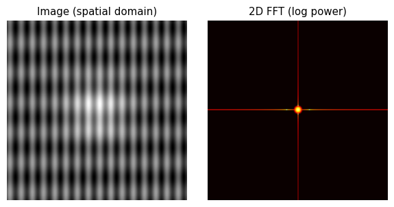
Bright spots in the FFT correspond to dominant spatial frequencies:
  - Center: DC component (average brightness)
  - Horizontal pair: vertical stripes
  - Vertical pair: horizontal stripes
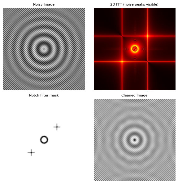
# Image denoising: remove periodic noise
# Create a clean image (concentric rings)
R = np.sqrt(X**2 + Y**2)
clean_image = np.sin(2 * np.pi * 5 * R) * np.exp(-R**2 / 0.5)

# Add periodic noise (diagonal stripes)
np.random.seed(42)
periodic_noise = 0.8 * np.sin(2 * np.pi * (20 * X + 20 * Y))
noisy_image = clean_image + periodic_noise

# 2D FFT
F_noisy = np.fft.fft2(noisy_image)
F_noisy_shifted = np.fft.fftshift(F_noisy)

# Identify and remove the noise peaks
# The periodic noise creates bright spots at specific spatial frequencies
power = np.abs(F_noisy_shifted)

# Create a mask: suppress points far from center that are unusually bright
ky = np.arange(M) - M//2
kx = np.arange(N_img) - N_img//2
KX, KY = np.meshgrid(kx, ky)
K_radius = np.sqrt(KX**2 + KY**2)

# Notch filter: remove the noise peaks (at diagonal positions)
mask = np.ones_like(power)
# Find peaks away from center
threshold = np.percentile(power[K_radius > 5], 99.5)
mask[(power > threshold) & (K_radius > 5)] = 0

# Smooth the mask slightly to avoid ringing
from scipy.ndimage import gaussian_filter
mask_smooth = gaussian_filter(mask, sigma=1)

# Apply mask and inverse FFT
F_cleaned = F_noisy_shifted * mask_smooth
cleaned_image = np.real(np.fft.ifft2(np.fft.ifftshift(F_cleaned)))

# Plot
fig, axes = plt.subplots(2, 2, figsize=(6, 6))

axes[0, 0].imshow(noisy_image, cmap='gray', origin='lower')
axes[0, 0].set_title('Noisy Image', fontsize=8)
axes[0, 0].axis('off')

axes[0, 1].imshow(np.log10(power + 1), cmap='hot', origin='lower')
axes[0, 1].set_title('2D FFT (noise peaks visible)', fontsize=8)
axes[0, 1].axis('off')

axes[1, 0].imshow(mask_smooth, cmap='gray', origin='lower')
axes[1, 0].set_title('Notch filter mask', fontsize=8)
axes[1, 0].axis('off')

axes[1, 1].imshow(cleaned_image, cmap='gray', origin='lower')
axes[1, 1].set_title('Cleaned Image', fontsize=8)
axes[1, 1].axis('off')

plt.tight_layout()
plt.show()
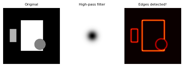
# Edge detection via high-pass filter in frequency domain
# Create a test image with sharp features
image_sharp = np.zeros((256, 256))
image_sharp[60:200, 80:180] = 1.0   # Rectangle
image_sharp[100:160, 30:60] = 0.7   # Small rectangle
# Add a circle
R_circle = np.sqrt((X - 0.3)**2 + (Y + 0.3)**2)
image_sharp[R_circle < 0.2] = 0.5

# 2D FFT
F_sharp = np.fft.fft2(image_sharp)
F_sharp_shifted = np.fft.fftshift(F_sharp)

# High-pass filter: remove low frequencies (keep edges)
hp_mask = 1 - np.exp(-(KX**2 + KY**2) / (2 * 15**2))  # Gaussian high-pass

F_edges = F_sharp_shifted * hp_mask
edges = np.real(np.fft.ifft2(np.fft.ifftshift(F_edges)))

fig, axes = plt.subplots(1, 3, figsize=(6, 2.5))

axes[0].imshow(image_sharp, cmap='gray', origin='lower')
axes[0].set_title('Original', fontsize=8)
axes[0].axis('off')

axes[1].imshow(hp_mask, cmap='gray', origin='lower')
axes[1].set_title('High-pass filter', fontsize=8)
axes[1].axis('off')

axes[2].imshow(np.abs(edges), cmap='hot', origin='lower')
axes[2].set_title('Edges detected!', fontsize=8)
axes[2].axis('off')

plt.tight_layout()
plt.show()
VII. Physics Applications#
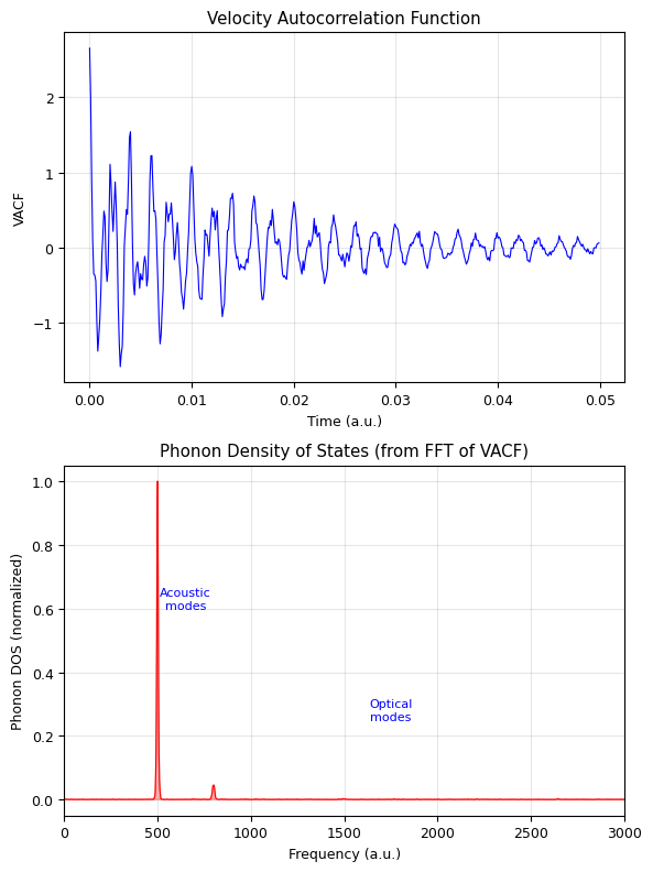
Application 1: Phonon Spectrum from Molecular Dynamics#
In computational materials science, we simulate atomic vibrations and use the FFT to extract the phonon density of states — the distribution of vibrational frequencies in a crystal.
# Simulated velocity autocorrelation function (VACF) of atoms in a crystal
# The FFT of the VACF gives the phonon density of states

fs = 10000  # sampling rate (arbitrary units, ~femtoseconds)
N = 4096
t = np.arange(N) / fs

# Simulated VACF: decaying oscillations at characteristic phonon frequencies
# Acoustic modes: low frequency (~500, 800 THz)
# Optical modes: higher frequency (~1500, 2000 THz)
np.random.seed(42)
vacf = (1.0 * np.cos(2 * np.pi * 500 * t) * np.exp(-t * 50) +
        0.8 * np.cos(2 * np.pi * 800 * t) * np.exp(-t * 80) +
        0.5 * np.cos(2 * np.pi * 1500 * t) * np.exp(-t * 120) +
        0.3 * np.cos(2 * np.pi * 2000 * t) * np.exp(-t * 150) +
        0.1 * np.random.randn(N) * np.exp(-t * 30))

# Apply Hann window to reduce leakage
window = signal.windows.hann(N)
vacf_windowed = vacf * window

# FFT to get phonon DOS
F = np.fft.rfft(vacf_windowed)
freqs = np.fft.rfftfreq(N, d=1/fs)
dos = np.abs(F)**2  # Power spectrum = phonon DOS

fig, (ax1, ax2) = plt.subplots(2, 1, figsize=(6, 8))

ax1.plot(t[:500], vacf[:500], 'b-', linewidth=0.8)
ax1.set_xlabel('Time (a.u.)')
ax1.set_ylabel('VACF')
ax1.set_title('Velocity Autocorrelation Function')
ax1.grid(True, alpha=0.3)

ax2.fill_between(freqs, dos / dos.max(), alpha=0.3, color='red')
ax2.plot(freqs, dos / dos.max(), 'r-', linewidth=0.8)
ax2.set_xlabel('Frequency (a.u.)')
ax2.set_ylabel('Phonon DOS (normalized)')
ax2.set_title('Phonon Density of States (from FFT of VACF)')
ax2.set_xlim(0, 3000)
ax2.grid(True, alpha=0.3)

# Annotate peaks
ax2.annotate('Acoustic\nmodes', xy=(650, 0.6), fontsize=8, ha='center', color='blue')
ax2.annotate('Optical\nmodes', xy=(1750, 0.25), fontsize=8, ha='center', color='blue')

plt.tight_layout()
plt.show()
Application 2: Gravitational Wave — Chirp Signal#
Gravitational waves from merging black holes produce a chirp: a signal whose frequency increases over time. We need the Short-Time Fourier Transform (STFT) to see how frequency evolves.
# Simulated gravitational wave chirp
fs = 4096  # Hz (typical GW detector sampling rate)
T = 2.0    # seconds before merger
N = int(fs * T)
t = np.linspace(0, T, N, endpoint=False)

# Chirp: frequency increases from 35 Hz to 250 Hz
f0 = 35   # starting frequency
f1 = 250  # ending frequency
# Phase: integral of instantaneous frequency
phase = 2 * np.pi * (f0 * t + (f1 - f0) / (2 * T) * t**2)
# Amplitude increases as merger approaches
amplitude = (1 - t / T)**(-0.25)
amplitude = np.clip(amplitude, 0, 10)  # prevent divergence

gw_signal = amplitude * np.sin(phase)

# Add detector noise
np.random.seed(42)
gw_noisy = gw_signal + 2 * np.random.randn(N)

# Spectrogram (STFT) — shows frequency vs time
freqs_stft, times_stft, Sxx = signal.spectrogram(
    gw_noisy, fs=fs, nperseg=256, noverlap=250, window='hann'
)

fig, axes = plt.subplots(3, 1, figsize=(6, 10))

# Time domain
axes[0].plot(t, gw_noisy, 'gray', linewidth=0.3, alpha=0.5, label='Noisy')
axes[0].plot(t, gw_signal, 'b-', linewidth=0.8, label='True signal')
axes[0].set_xlabel('Time before merger (s)')
axes[0].set_ylabel('Strain')
axes[0].set_title('Gravitational Wave Chirp')
axes[0].legend(fontsize=7)
axes[0].grid(True, alpha=0.3)

# Regular FFT (loses time information)
F_gw = np.fft.rfft(gw_noisy)
f_gw = np.fft.rfftfreq(N, d=1/fs)
axes[1].plot(f_gw, np.abs(F_gw), 'r-', linewidth=0.5)
axes[1].set_xlim(0, 400)
axes[1].set_xlabel('Frequency (Hz)')
axes[1].set_ylabel('|F(f)|')
axes[1].set_title('Regular FFT (frequency info, but no timing!)')
axes[1].grid(True, alpha=0.3)

# Spectrogram
axes[2].pcolormesh(times_stft, freqs_stft, 10 * np.log10(Sxx + 1e-10),
                   shading='gouraud', cmap='magma')
axes[2].set_ylim(0, 400)
axes[2].set_xlabel('Time (s)')
axes[2].set_ylabel('Frequency (Hz)')
axes[2].set_title('Spectrogram (STFT) — frequency evolves over time!')

plt.tight_layout()
plt.show()

print("The spectrogram reveals the chirp: frequency sweeping from ~35 to ~250 Hz!")
print("Regular FFT shows all frequencies present, but not WHEN they occur.")
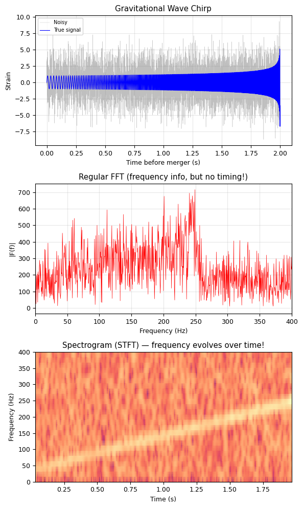
The spectrogram reveals the chirp: frequency sweeping from ~35 to ~250 Hz!
Regular FFT shows all frequencies present, but not WHEN they occur.
Application: Solving PDEs with FFT (Spectral Methods)#
The FFT turns derivatives into multiplication in frequency space:
This makes solving differential equations extremely fast — known as spectral methods.
We’ll cover PDEs in detail in our PDE lectures.