Numerical Differentiation

Why Numerical Differentiation?

• The function is only known at discrete data points (experimental measurements)

• The analytical derivative is too complex to compute

• We need to verify analytical results computationally

• Building blocks for solving differential equations

import numpy as np
import matplotlib.pyplot as plt
from scipy.interpolate import UnivariateSpline
from scipy.signal import savgol_filter

# For nicer plots
plt.rcParams['figure.figsize'] = [5, 3]
plt.rcParams['font.size'] = 12

I. The Differentiation Problem

We want to compute the derivative:

\[f'(x) = \lim_{h \to 0} \frac{f(x+h) - f(x)}{h}\]

The challenge: we can’t take \(h \to 0\) on a computer! We must use a finite value of \(h\).

The Fundamental Trade-off

• Too large h: Poor approximation (truncation error)

• Too small h: Numerical noise dominates (round-off error)

Finding the right \(h\) is key to accurate numerical differentiation.

# Visualize the derivative as a limit
def f(x):
    return np.sin(x)

def f_prime_exact(x):
    return np.cos(x)

x0 = np.pi/4  # Point where we compute derivative
x = np.linspace(0, np.pi/2, 100)

plt.figure(figsize=(5, 8))

plt.subplot(2, 1, 1)
plt.plot(x, f(x), 'b-', linewidth=2, label=r'$f(x) = \sin(x)$')

# Show secant lines for different h
for h, color in [(0.5, 'red'), (0.25, 'orange'), (0.1, 'green')]:
    slope = (f(x0 + h) - f(x0)) / h
    y_secant = f(x0) + slope * (x - x0)
    plt.plot(x, y_secant, color=color, linestyle='--',
             label=f'Secant h={h}: slope={slope:.4f}')

# Tangent line (true derivative)
slope_true = f_prime_exact(x0)
y_tangent = f(x0) + slope_true * (x - x0)
plt.plot(x, y_tangent, 'k-', linewidth=2, label=f'Tangent: slope={slope_true:.4f}')

plt.plot(x0, f(x0), 'ko', markersize=10)
plt.xlabel('x')
plt.ylabel('f(x)')
plt.title(r'Derivative at $x = \pi/4$')
plt.legend(loc='upper left')
plt.grid(True, alpha=0.3)
plt.ylim(0, 1.5)

plt.subplot(2, 1, 2)
# Error as function of h
h_values = np.logspace(-15, 0, 100)
errors = np.abs((f(x0 + h_values) - f(x0)) / h_values - f_prime_exact(x0))

plt.loglog(h_values, errors, 'b-', linewidth=2)
plt.xlabel('h')
plt.ylabel('Absolute Error')
plt.title('Error in Forward Difference')
plt.grid(True, alpha=0.3)

# Mark optimal region
optimal_h = h_values[np.argmin(errors)]
plt.axvline(optimal_h, color='r', linestyle='--', label=f'Optimal h ≈ {optimal_h:.0e}')
plt.legend()

plt.tight_layout()
plt.show()

print(f"True derivative at x = π/4: {f_prime_exact(x0):.10f}")
print(f"Optimal h: {optimal_h:.2e}")
print(f"Minimum error: {errors.min():.2e}")

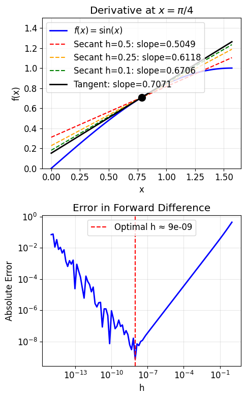
True derivative at x = π/4: 0.7071067812
Optimal h: 9.33e-09
Minimum error: 7.46e-10

II. Finite Difference Approximations

The three basic finite difference formulas:

Forward Difference

\[f'(x) \approx \frac{f(x+h) - f(x)}{h}\]

Backward Difference

\[f'(x) \approx \frac{f(x) - f(x-h)}{h}\]

Central Difference

\[f'(x) \approx \frac{f(x+h) - f(x-h)}{2h}\]

The central difference is more accurate because errors cancel!

def forward_diff(f, x, h):
    """Forward difference approximation of f'(x)."""
    return (f(x + h) - f(x)) / h

def backward_diff(f, x, h):
    """Backward difference approximation of f'(x)."""
    return (f(x) - f(x-h)) / h

def central_diff(f, x, h):
    """Central difference approximation of f'(x)."""
    return (f(x+h) - f(x-h)) / (2*h)

# Compare the three methods
def f(x):
    return np.exp(x)

def f_prime(x):
    return np.exp(x)  # Derivative of e^x is e^x

x0 = 1.0
true_value = f_prime(x0)

print("Comparison of Finite Difference Methods")
print(f"Function: f(x) = e^x at x = {x0}")
print(f"True derivative: {true_value:.10f}")
print("=" * 70)
print(f"{'h':>12} {'Forward':>15} {'Backward':>15} {'Central':>15}")
print("-" * 70)

for h in [0.1, 0.01, 0.001, 0.0001, 0.00001]:
    fwd = forward_diff(f, x0, h)
    bwd = backward_diff(f, x0, h)
    ctr = central_diff(f, x0, h)

    err_fwd = abs(fwd - true_value)
    err_bwd = abs(bwd - true_value)
    err_ctr = abs(ctr - true_value)

    print(f"{h:>12.0e} {err_fwd:>15.2e} {err_bwd:>15.2e} {err_ctr:>15.2e}")

print("\nObservation: Central difference is MUCH more accurate!")

Comparison of Finite Difference Methods
Function: f(x) = e^x at x = 1.0
True derivative: 2.7182818285
======================================================================
           h         Forward        Backward         Central
----------------------------------------------------------------------
       1e-01        1.41e-01        1.31e-01        4.53e-03
       1e-02        1.36e-02        1.35e-02        4.53e-05
       1e-03        1.36e-03        1.36e-03        4.53e-07
       1e-04        1.36e-04        1.36e-04        4.53e-09
       1e-05        1.36e-05        1.36e-05        5.86e-11

Observation: Central difference is MUCH more accurate!

Why is Central Difference Better?

Using Taylor series expansion:

Forward difference: $\(f(x+h) = f(x) + hf'(x) + \frac{h^2}{2}f''(x) + O(h^3)\)$

\[\frac{f(x+h) - f(x)}{h} = f'(x) + \frac{h}{2}f''(x) + O(h^2)\]

Error is \(O(h)\) — first-order accurate

Central difference: $\(f(x+h) = f(x) + hf'(x) + \frac{h^2}{2}f''(x) + \frac{h^3}{6}f'''(x) + O(h^4)\)\( \)\(f(x-h) = f(x) - hf'(x) + \frac{h^2}{2}f''(x) - \frac{h^3}{6}f'''(x) + O(h^4)\)$

\[\frac{f(x+h) - f(x-h)}{2h} = f'(x) + \frac{h^2}{6}f'''(x) + O(h^4)\]

Error is \(O(h^2)\) — second-order accurate

# Visualize convergence rates
def f(x):
    return np.sin(x)

def f_prime(x):
    return np.cos(x)

x0 = 1.0
true_value = f_prime(x0)

h_values = np.logspace(-10, -1, 50)
errors_fwd = np.abs(forward_diff(f, x0, h_values) - true_value)
errors_bwd = np.abs(backward_diff(f, x0, h_values) - true_value)
errors_ctr = np.abs(central_diff(f, x0, h_values) - true_value)

plt.figure(figsize=(5, 6))
plt.loglog(h_values, errors_fwd, 'b-', linewidth=2, label='Forward Difference')
plt.loglog(h_values, errors_bwd, 'g--', linewidth=2, label='Backward Difference')
plt.loglog(h_values, errors_ctr, 'r-', linewidth=2, label='Central Difference')

# Reference lines
plt.loglog(h_values, h_values, 'k:', alpha=0.5, label=r'$O(h)$ reference')
plt.loglog(h_values, h_values**2, 'k--', alpha=0.5, label=r'$O(h^2)$ reference')

plt.xlabel('h')
plt.ylabel('Absolute Error')
plt.title('Convergence of Finite Difference Methods')
plt.legend()
plt.grid(True, alpha=0.3)
plt.show()

print("Notice:")
print("- Forward/Backward follow the O(h) line (slope = 1)")
print("- Central follows the O(h²) line (slope = 2)")
print("- At very small h, round-off error takes over!")

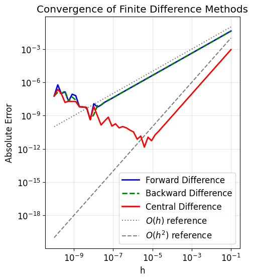
Notice:
- Forward/Backward follow the O(h) line (slope = 1)
- Central follows the O(h²) line (slope = 2)
- At very small h, round-off error takes over!

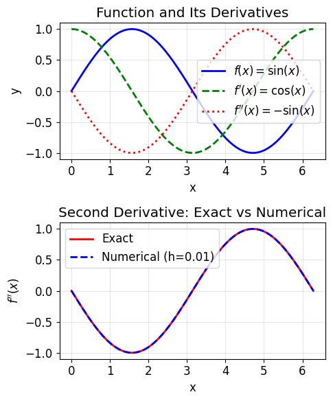
III. Second Derivatives

For the second derivative, we can use the central difference formula:

\[f''(x) \approx \frac{f(x+h) - 2f(x) + f(x-h)}{h^2}\]

This is derived by combining forward and backward differences, or by Taylor expansion.

This formula is \(O(h^2)\) accurate.

def second_derivative(f, x, h):
    """Central difference approximation of f''(x)."""
    # finish this function...
    return (f(x+h) - 2*f(x) + f(x-h))/h**2

# Test with f(x) = sin(x), f''(x) = -sin(x)
def f(x):
    return np.sin(x)
    # return np.exp(x)

def f_double_prime(x):
    return -np.sin(x)
    # return np.exp(x)

x0 = np.pi/3
true_value = f_double_prime(x0)

print("Second Derivative Approximation")
print(f"Function: f(x) = sin(x) at x = π/3")
print(f"True f''(x): {true_value:.10f}")
print("=" * 50)
print(f"{'h':>12} {'Approximation':>18} {'Error':>15}")
print("-" * 50)

for h in [0.1, 0.01, 0.001, 0.0001, 0.00001, 0.000001]:
    approx = second_derivative(f, x0, h)
    error = abs(approx - true_value)
    print(f"{h:>12.0e} {approx:>18.10f} {error:>15.2e}")

print("\nNote: Very small h causes round-off errors (dividing by h²!)")

Second Derivative Approximation
Function: f(x) = sin(x) at x = π/3
True f''(x): -0.8660254038
==================================================
           h      Approximation           Error
--------------------------------------------------
       1e-01      -0.8653039565        7.21e-04
       1e-02      -0.8660181869        7.22e-06
       1e-03      -0.8660253317        7.21e-08
       1e-04      -0.8660253958        7.94e-09
       1e-05      -0.8660250295        3.74e-07
       1e-06      -0.8659739592        5.14e-05

Note: Very small h causes round-off errors (dividing by h²!)

# Visualize second derivative calculation
x = np.linspace(0, 2*np.pi, 200)
y = np.sin(x)

# Compute numerical second derivative
h = 0.01
y_double_prime_numerical = second_derivative(np.sin, x, h)
y_double_prime_exact = -np.sin(x)

plt.figure(figsize=(5, 6))

plt.subplot(2, 1, 1)
plt.plot(x, y, 'b-', linewidth=2, label=r"$f(x) = \sin(x)$")
plt.plot(x, np.cos(x), 'g--', linewidth=2, label=r"$f'(x) = \cos(x)$")
plt.plot(x, -np.sin(x), 'r:', linewidth=2, label=r"$f''(x) = -\sin(x)$")
plt.xlabel('x')
plt.ylabel('y')
plt.title('Function and Its Derivatives')
plt.legend()
plt.grid(True, alpha=0.3)

plt.subplot(2, 1, 2)
plt.plot(x, y_double_prime_exact, 'r-', linewidth=2, label='Exact')
plt.plot(x, y_double_prime_numerical, 'b--', linewidth=2, label=f'Numerical (h={h})')
plt.xlabel('x')
plt.ylabel(r"$f''(x)$")
plt.title('Second Derivative: Exact vs Numerical')
plt.legend()
plt.grid(True, alpha=0.3)

plt.tight_layout()
plt.show()

IV. Error Analysis: The Optimal Step Size

Numerical differentiation faces two competing errors:

1. Truncation Error

From truncating the Taylor series. Decreases as \(h\) decreases.

• Forward/Backward: \(\sim \frac{h}{2}|f''(x)|\)

• Central: \(\sim \frac{h^2}{6}|f'''(x)|\)

2. Round-off Error

From finite precision arithmetic. Increases as \(h\) decreases!

When subtracting nearly equal numbers: \(f(x+h) \approx f(x)\) for small \(h\).

Round-off error \(\sim \frac{\epsilon |f(x)|}{h}\) where \(\epsilon \approx 10^{-16}\) for double precision.

Optimal h

For central difference, balancing truncation and round-off:

\[h_{opt} \sim \epsilon^{1/3} \approx 10^{-5} \text{ to } 10^{-6}\]

# Demonstrate the truncation vs round-off trade-off
def f(x):
    return np.exp(x)

def f_prime(x):
    return np.exp(x)

x0 = 1.0
true_value = f_prime(x0)

h_values = np.logspace(-16, 0, 100)
errors_fwd = np.abs(forward_diff(f, x0, h_values) - true_value)
errors_ctr = np.abs(central_diff(f, x0, h_values) - true_value)

# Find optimal h
opt_h_fwd = h_values[np.argmin(errors_fwd)]
opt_h_ctr = h_values[np.argmin(errors_ctr)]

plt.figure(figsize=(5, 6))
plt.loglog(h_values, errors_fwd, 'b-', linewidth=2, label='Forward Difference')
plt.loglog(h_values, errors_ctr, 'r-', linewidth=2, label='Central Difference')

plt.axvline(opt_h_fwd, color='b', linestyle='--', alpha=0.7,
            label=f'Optimal h (forward) ≈ {opt_h_fwd:.0e}')
plt.axvline(opt_h_ctr, color='r', linestyle='--', alpha=0.7,
            label=f'Optimal h (central) ≈ {opt_h_ctr:.0e}')

# Annotate regions
plt.annotate('Truncation\nerror\ndominates', xy=(1e-2, 1e-4), fontsize=10,
             ha='center', bbox=dict(boxstyle='round', facecolor='wheat'))
plt.annotate('Round-off\nerror\ndominates', xy=(1e-14, 1e-4), fontsize=10,
             ha='center', bbox=dict(boxstyle='round', facecolor='wheat'))

plt.xlabel('h')
plt.ylabel('Absolute Error')
plt.title('Error in Numerical Differentiation: The Optimal h')
plt.legend(loc='upper right')
plt.grid(True, alpha=0.3)
plt.ylim(1e-12, 1)
plt.show()

print(f"Optimal h for forward difference: {opt_h_fwd:.2e}")
print(f"Minimum error: {errors_fwd.min():.2e}")
print(f"\nOptimal h for central difference: {opt_h_ctr:.2e}")
print(f"Minimum error: {errors_ctr.min():.2e}")
print(f"\nCentral difference achieves ~{errors_fwd.min()/errors_ctr.min():.0f}x better accuracy!")

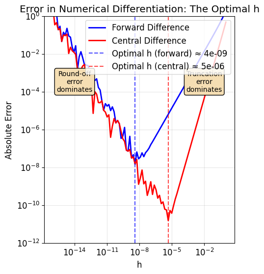
Optimal h for forward difference: 3.94e-09
Minimum error: 1.46e-08

Optimal h for central difference: 4.64e-06
Minimum error: 1.53e-11

Central difference achieves ~960x better accuracy!

V. Higher-Order Formulas

We can improve accuracy by using more points. These are derived from Taylor series or polynomial interpolation.

Fourth-Order Central Difference (5-point stencil)

\[f'(x) \approx \frac{-f(x+2h) + 8f(x+h) - 8f(x-h) + f(x-2h)}{12h}\]

Error is \(O(h^4)\) — much better than basic central difference!

Fourth-Order Second Derivative

\[f''(x) \approx \frac{-f(x+2h) + 16f(x+h) - 30f(x) + 16f(x-h) - f(x-2h)}{12h^2}\]

def central_diff_4th_order(f, x, h):
    """Fourth-order central difference approximation of f'(x)."""
    return (-f(x + 2*h) + 8*f(x + h) - 8*f(x - h) + f(x - 2*h)) / (12 * h)

def second_deriv_4th_order(f, x, h):
    """Fourth-order central difference approximation of f''(x)."""
    return (-f(x + 2*h) + 16*f(x + h) - 30*f(x) + 16*f(x - h) - f(x - 2*h)) / (12 * h**2)

# Compare second-order vs fourth-order
def f(x):
    return np.sin(x)

def f_prime(x):
    return np.cos(x)

x0 = 1.0
true_value = f_prime(x0)

print("Comparison: 2nd-Order vs 4th-Order Central Difference")
print(f"Function: f(x) = sin(x) at x = {x0}")
print(f"True f'(x): {true_value:.15f}")
print("=" * 60)
print(f"{'h':>10} {'2nd-Order Error':>20} {'4th-Order Error':>20}")
print("-" * 60)

for h in [0.1, 0.05, 0.02, 0.01, 0.005]:
    err_2nd = abs(central_diff(f, x0, h) - true_value)
    err_4th = abs(central_diff_4th_order(f, x0, h) - true_value)
    print(f"{h:>10.3f} {err_2nd:>20.2e} {err_4th:>20.2e}")

print("\n4th-order is dramatically more accurate!")

Comparison: 2nd-Order vs 4th-Order Central Difference
Function: f(x) = sin(x) at x = 1.0
True f'(x): 0.540302305868140
============================================================
         h      2nd-Order Error      4th-Order Error
------------------------------------------------------------
     0.100             9.00e-04             1.80e-06
     0.050             2.25e-04             1.13e-07
     0.020             3.60e-05             2.88e-09
     0.010             9.00e-06             1.80e-10
     0.005             2.25e-06             1.13e-11

4th-order is dramatically more accurate!

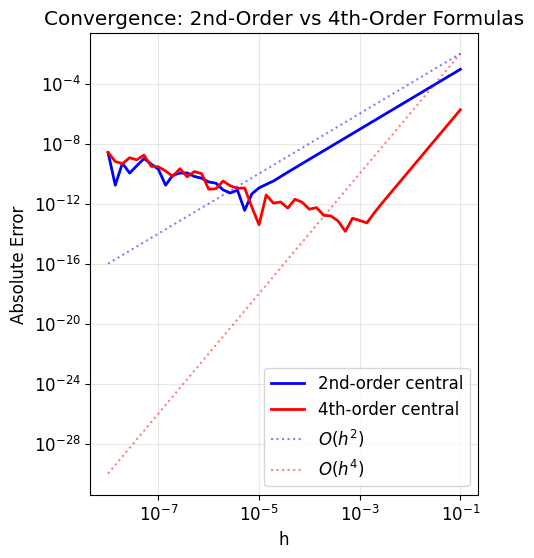
# Visualize convergence of different orders
h_values = np.logspace(-8, -1, 50)

errors_2nd = np.abs(central_diff(f, x0, h_values) - true_value)
errors_4th = np.abs(central_diff_4th_order(f, x0, h_values) - true_value)

plt.figure(figsize=(5, 6))
plt.loglog(h_values, errors_2nd, 'b-', linewidth=2, label='2nd-order central')
plt.loglog(h_values, errors_4th, 'r-', linewidth=2, label='4th-order central')

# Reference lines
plt.loglog(h_values, h_values**2, 'b:', alpha=0.5, label=r'$O(h^2)$')
plt.loglog(h_values, h_values**4 * 100, 'r:', alpha=0.5, label=r'$O(h^4)$')

plt.xlabel('h')
plt.ylabel('Absolute Error')
plt.title('Convergence: 2nd-Order vs 4th-Order Formulas')
plt.legend()
plt.grid(True, alpha=0.3)
plt.show()

print("Observation:")
print("- 2nd-order: halving h reduces error by 4x")
print("- 4th-order: halving h reduces error by 16x!")

Observation:
- 2nd-order: halving h reduces error by 4x
- 4th-order: halving h reduces error by 16x!

VI. Derivatives from Data

In experimental physics, we often have data points \((x_i, y_i)\) rather than a function.

Approaches:

1. Direct finite differences — Simple but noisy

2. Fit a smooth function — Then differentiate analytically

3. Spline interpolation — Smooth and flexible

4. Savitzky-Golay filter — Smoothing + differentiation

# Generate noisy experimental data
np.random.seed(42)

# True function
def true_func(x):
    return np.sin(2 * x)

def true_derivative(x):
    return 2 * np.cos(2 * x)

# Simulated experimental data
x_data = np.linspace(0, 2*np.pi, 30)
y_data = true_func(x_data) + 0.1 * np.random.randn(len(x_data))  # Add noise

# Method 1: Direct finite differences
dy_direct = np.diff(y_data) / np.diff(x_data)
x_direct = (x_data[:-1] + x_data[1:]) / 2  # Midpoints

# Method 2: Central differences (for interior points)
dy_central = (y_data[2:] - y_data[:-2]) / (x_data[2:] - x_data[:-2])
x_central = x_data[1:-1]

# Method 3: Spline interpolation
spline = UnivariateSpline(x_data, y_data, s=0.5)  # s controls smoothing
x_fine = np.linspace(0, 2*np.pi, 200)
dy_spline = spline.derivative()(x_fine)

# Plot results
plt.figure(figsize=(6, 8))

plt.subplot(2, 1, 1)
plt.plot(x_data, y_data, 'ko', markersize=6, label='Noisy data')
plt.plot(x_fine, true_func(x_fine), 'b-', linewidth=2, label='True function')
plt.plot(x_fine, spline(x_fine), 'r--', linewidth=2, label='Spline fit')
plt.xlabel('x')
plt.ylabel('y')
plt.title('Original Data and Fits')
plt.legend()
plt.grid(True, alpha=0.3)

plt.subplot(2, 1, 2)
plt.plot(x_fine, true_derivative(x_fine), 'b-', linewidth=2, label='True derivative')
plt.plot(x_direct, dy_direct, 'g.-', alpha=0.7, label='Direct differences (noisy!)')
plt.plot(x_fine, dy_spline, 'r--', linewidth=2, label='Spline derivative (smooth)')
plt.xlabel('x')
plt.ylabel("y'")
plt.title('Derivative Estimates')
plt.legend()
plt.grid(True, alpha=0.3)

plt.tight_layout()
plt.show()

print("Key insight: Direct finite differences amplify noise!")
print("Spline interpolation provides a much smoother derivative.")

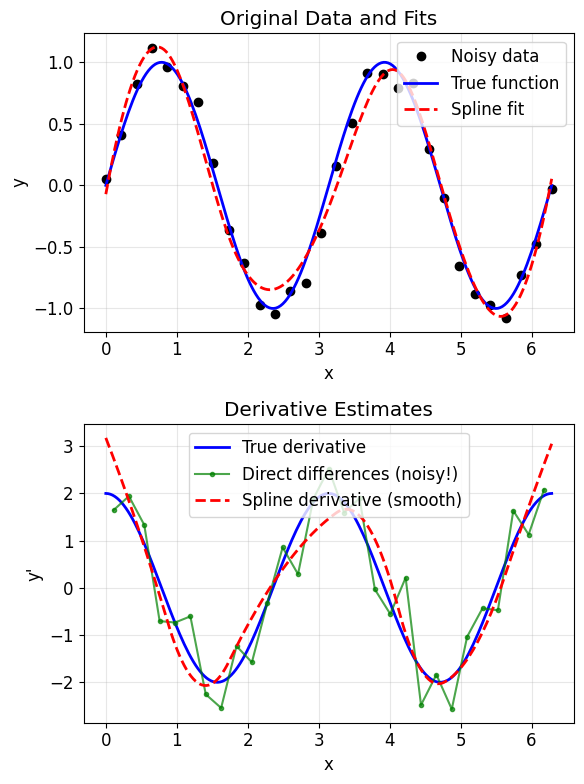
Key insight: Direct finite differences amplify noise!
Spline interpolation provides a much smoother derivative.

Savitzky-Golay Filter

A popular method that simultaneously smooths data AND computes derivatives.

It fits a polynomial to a moving window and extracts the derivative from the polynomial coefficients.

We will cover this next week.

VII. Using np.gradient() for Array Data

For arrays of data, NumPy’s np.gradient() is the go-to tool:

• Computes centered differences for interior points

• Handles edges automatically (uses forward/backward differences)

• Works with non-uniform spacing

# Example: Using np.gradient for derivatives
def f(x):
    return x**3 * np.exp(-x)

x = np.linspace(0, 4, 100)
y = f(x)

# np.gradient computes centered differences, handling edges appropriately
# Syntax: np.gradient(y, x) where x is the coordinate array
dy = np.gradient(y, x)   # First derivative
ddy = np.gradient(dy, x) # Second derivative (apply gradient twice)

# Exact derivatives for comparison
# f(x) = x³e^(-x)
# f'(x) = x²e^(-x)(3-x)
# f''(x) = e^(-x)(x² - 6x + 6)
dy_exact = x**2 * np.exp(-x) * (3 - x)
ddy_exact = np.exp(-x) * (x**2 - 6*x + 6)

plt.figure(figsize=(5, 6))

plt.subplot(2, 1, 1)
plt.plot(x, y, 'b-', linewidth=2, label=r'$f(x) = x^3 e^{-x}$')
plt.plot(x, dy, 'r--', linewidth=2, label=r"$f'(x)$ numerical")
plt.plot(x, dy_exact, 'g:', linewidth=2, label=r"$f'(x)$ exact")
plt.xlabel('x')
plt.ylabel('y')
plt.title('Function and First Derivative')
plt.legend()
plt.grid(True, alpha=0.3)

plt.subplot(2, 1, 2)
plt.plot(x, ddy, 'r--', linewidth=2, label=r"$f''(x)$ numerical")
plt.plot(x, ddy_exact, 'g:', linewidth=2, label=r"$f''(x)$ exact")
plt.xlabel('x')
plt.ylabel('y')
plt.title('Second Derivative')
plt.legend()
plt.grid(True, alpha=0.3)

plt.tight_layout()
plt.show()

# Show the error
print("Maximum error in first derivative:", np.max(np.abs(dy - dy_exact)))
print("Maximum error in second derivative:", np.max(np.abs(ddy - ddy_exact)))

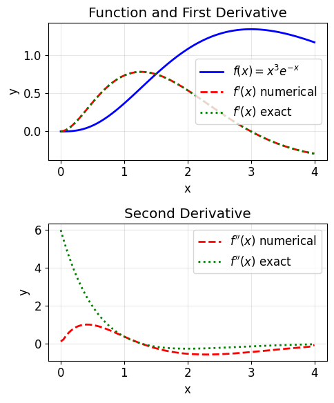
Maximum error in first derivative: 0.0030302710209441086
Maximum error in second derivative: 5.889734082400933

VIII. Physics Applications

Let’s apply numerical differentiation to real physics problems!

1. Heat Transfer: Temperature Gradient

The heat flux is proportional to the temperature gradient (Fourier’s Law):

\[q = -k \frac{dT}{dx}\]

where \(k\) is the thermal conductivity.

# Temperature distribution in a rod with heat source
# Steady state: k*d²T/dx² + Q = 0
# Solution with T(0)=T(L)=T0: T(x) = T0 + (Q/2k)*x*(L-x)

L = 1.0       # Rod length (m)
T0 = 300      # Boundary temperature (K)
k_thermal = 50  # Thermal conductivity (W/m·K)
Q = 1000      # Heat source (W/m³)

x = np.linspace(0, L, 50)

# Temperature distribution
T = T0 + (Q / (2 * k_thermal)) * x * (L - x)

# Temperature gradient dT/dx
dT_dx = np.gradient(T, x)
dT_dx_exact = (Q / (2 * k_thermal)) * (L - 2*x)

# Heat flux q = -k dT/dx
q = -k_thermal * dT_dx

plt.figure(figsize=(12, 4))

plt.subplot(1, 3, 1)
plt.plot(x, T, 'r-', linewidth=2)
plt.xlabel('Position x (m)')
plt.ylabel('Temperature T (K)')
plt.title('Temperature Distribution')
plt.grid(True, alpha=0.3)

plt.subplot(1, 3, 2)
plt.plot(x, dT_dx, 'b-', linewidth=2, label='Numerical')
plt.plot(x, dT_dx_exact, 'g--', linewidth=2, label='Exact')
plt.xlabel('Position x (m)')
plt.ylabel('dT/dx (K/m)')
plt.title('Temperature Gradient')
plt.legend()
plt.grid(True, alpha=0.3)

plt.subplot(1, 3, 3)
plt.plot(x, q, 'purple', linewidth=2)
plt.axhline(0, color='k', linestyle='-', linewidth=0.5)
plt.xlabel('Position x (m)')
plt.ylabel('Heat flux q (W/m²)')
plt.title('Heat Flux: q = -k dT/dx')
plt.grid(True, alpha=0.3)

plt.tight_layout()
plt.show()

print("Observations:")
print("- Temperature peaks at the center (heat generated throughout rod)")
print("- Gradient is positive on left (heat flows left), negative on right (heat flows right)")
print("- Heat flows from center outward toward the cooled boundaries")

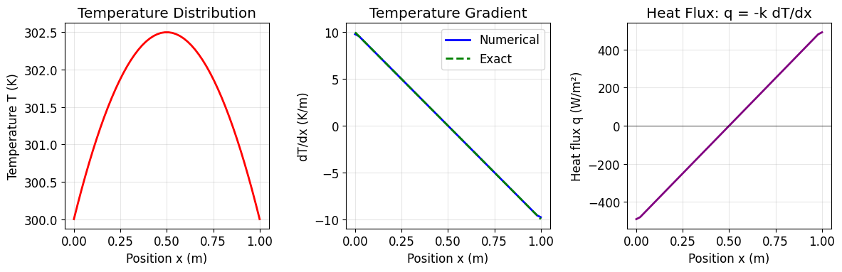
Observations:
- Temperature peaks at the center (heat generated throughout rod)
- Gradient is positive on left (heat flows left), negative on right (heat flows right)
- Heat flows from center outward toward the cooled boundaries

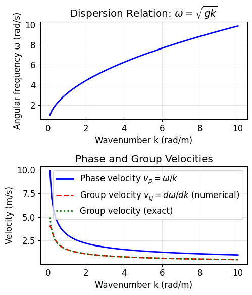
2. Wave Properties: Group Velocity

The group velocity of a wave packet is:

\[v_g = \frac{d\omega}{dk}\]

where \(\omega(k)\) is the dispersion relation.

# Dispersion relation for deep water waves: ω = √(gk)
g = 9.8  # m/s²

k = np.linspace(0.1, 10, 100)  # Wavenumber (rad/m)
omega = np.sqrt(g * k)  # Angular frequency (rad/s)

# Phase velocity: v_p = ω/k
v_phase = omega / k

# Group velocity: v_g = dω/dk
v_group_numerical = np.gradient(omega, k)

# Exact: v_g = d(√(gk))/dk = (1/2)√(g/k) = v_p/2
v_group_exact = 0.5 * np.sqrt(g / k)

plt.figure(figsize=(5, 6))

plt.subplot(2, 1, 1)
plt.plot(k, omega, 'b-', linewidth=2)
plt.xlabel('Wavenumber k (rad/m)')
plt.ylabel('Angular frequency ω (rad/s)')
plt.title(r'Dispersion Relation: $\omega = \sqrt{gk}$')
plt.grid(True, alpha=0.3)

plt.subplot(2, 1, 2)
plt.plot(k, v_phase, 'b-', linewidth=2, label='Phase velocity $v_p = ω/k$')
plt.plot(k, v_group_numerical, 'r--', linewidth=2, label='Group velocity $v_g = dω/dk$ (numerical)')
plt.plot(k, v_group_exact, 'g:', linewidth=2, label='Group velocity (exact)')
plt.xlabel('Wavenumber k (rad/m)')
plt.ylabel('Velocity (m/s)')
plt.title('Phase and Group Velocities')
plt.legend()
plt.grid(True, alpha=0.3)

plt.tight_layout()
plt.show()

print("Key insight: For deep water waves, v_group = v_phase / 2")
print("Energy travels at half the speed of the wave crests!")

Key insight: For deep water waves, v_group = v_phase / 2
Energy travels at half the speed of the wave crests!