Lecture 10: Ordinary Differential Equations (ODEs)#
Computational Physics — Spring 2026
Why ODEs?#
Almost every law of physics is a differential equation:
Physics |
Equation |
Type |
|---|---|---|
Newton’s 2nd law |
\(m\ddot{x} = F(x, \dot{x}, t)\) |
2nd order ODE |
Radioactive decay |
\(dN/dt = -\lambda N\) |
1st order ODE |
Damped oscillator |
\(m\ddot{x} + c\dot{x} + kx = 0\) |
2nd order ODE |
Heat diffusion (1D) |
\(\dot{T} = \alpha \, T''\) |
PDE → system of ODEs |
Crystal lattice vibrations |
\(m\ddot{u}_n = K(u_{n+1} - 2u_n + u_{n-1})\) |
System of ODEs |
import numpy as np
import matplotlib.pyplot as plt
from scipy.integrate import solve_ivp

# Projector-friendly settings
plt.rcParams['figure.figsize'] = [6, 4]
plt.rcParams['font.size'] = 9

print("Ready!")
Ready!
I. What Is an ODE?#
An ordinary differential equation relates a function to its derivatives:
Given an initial condition \(y(t_0) = y_0\), we want to find \(y(t)\) for \(t > t_0\).
Higher-order ODEs can always be rewritten as a system of first-order ODEs:
This is the standard form that all numerical solvers expect.
Slope Fields: Visualizing ODEs#
Before solving, we can visualize the ODE. At every point \((t, y)\), the derivative \(f(t, y)\) gives the slope.
# Slope field for dy/dt = -2*y + sin(t)
t_grid = np.linspace(0, 5, 20)
y_grid = np.linspace(-1.5, 1.5, 15)
T, Y = np.meshgrid(t_grid, y_grid)

def f_example(t, y):
    return -2 * y + np.sin(t)

dY = f_example(T, Y)
dT = np.ones_like(dY)  # dt component = 1
# Normalize arrows
norm = np.sqrt(dT**2 + dY**2)
dT /= norm
dY /= norm

fig, ax = plt.subplots(figsize=(6, 5))
ax.quiver(T, Y, dT, dY, color='steelblue', alpha=0.6, scale=30)

# Solve and overlay a few trajectories
for y0 in [-1.0, 0.0, 1.0]:
    sol = solve_ivp(f_example, [0, 5], [y0], t_eval=np.linspace(0, 5, 200))
    ax.plot(sol.t, sol.y[0], linewidth=1.5, label=f'y₀ = {y0}')

ax.set_xlabel('t')
ax.set_ylabel('y')
ax.set_title("Slope Field: dy/dt = -2y + sin(t)")
ax.legend(fontsize=7)
ax.grid(True, alpha=0.3)
plt.tight_layout()
plt.show()

print("All trajectories follow the arrows and converge to the same attractor!")
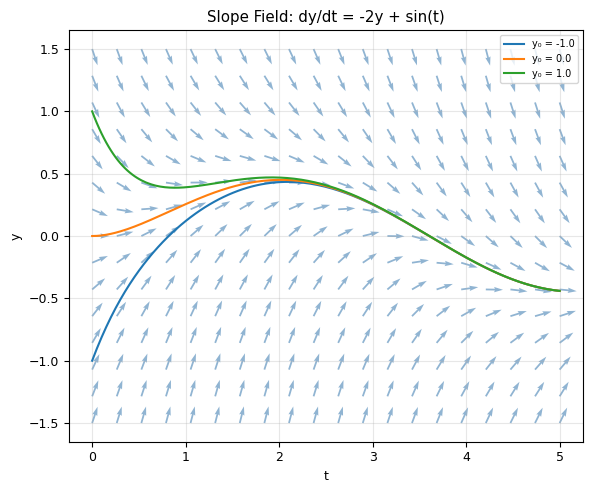
All trajectories follow the arrows and converge to the same attractor!
II. The Euler Method#
The Simplest Idea#
Approximate the derivative with a finite difference:
Rearranging:
Start at \((t_0, y_0)\)
Compute slope \(f(t_0, y_0)\)
Take a step: \(y_1 = y_0 + \Delta t \cdot f(t_0, y_0)\)
Repeat
Error per step: \(O(\Delta t^2)\) → Global error: \(O(\Delta t)\) — first-order method.
def euler(f, t_span, y0, dt):
    """Solve dy/dt = f(t, y) using Euler's method.

    Parameters
    ----------
    f : callable
        Right-hand side function f(t, y).
    t_span : tuple
        (t_start, t_end).
    y0 : array_like
        Initial condition (scalar or array).
    dt : float
        Time step.

    Returns
    -------
    t : ndarray
        Time points.
    y : ndarray
        Solution at each time point.
    """
    t_start, t_end = t_span
    t = np.arange(t_start, t_end + dt/2, dt)
    y0 = np.atleast_1d(np.array(y0, dtype=float))
    y = np.zeros((len(t), len(y0)))
    y[0] = y0

    for i in range(len(t) - 1):
        # y[i+1] =
        # code
        y[i+1] = y[i] + dt * np.array(f(t[i], y[i]))

    return t, y

# Test: exponential decay dy/dt = -y, y(0) = 1
# Exact solution: y = e^(-t)
t_euler, y_euler = euler(lambda t, y: -y, [0, 5], [1.0], dt=0.5)
t_exact = np.linspace(0, 5, 200)
y_exact = np.exp(-t_exact)

fig, ax = plt.subplots(figsize=(6, 5))
ax.plot(t_exact, y_exact, 'b-', linewidth=1.5, label='Exact: $e^{-t}$')
ax.plot(t_euler, y_euler[:, 0], 'ro--', markersize=5, label='Euler (Δt = 0.5)')

# Also show smaller dt
t_e2, y_e2 = euler(lambda t, y: -y, [0, 5], [1.0], dt=0.1)
ax.plot(t_e2, y_e2[:, 0], 'gs--', markersize=3, label='Euler (Δt = 0.1)')

ax.set_xlabel('t')
ax.set_ylabel('y')
ax.set_title('Euler Method: Exponential Decay')
ax.legend(fontsize=7)
ax.grid(True, alpha=0.3)
plt.tight_layout()
plt.show()

print(f"Error at t=5 (Δt=0.5): {abs(y_euler[-1, 0] - np.exp(-5)):.4f}")
print(f"Error at t=5 (Δt=0.1): {abs(y_e2[-1, 0] - np.exp(-5)):.4f}")
print(f"Ratio: {abs(y_euler[-1, 0] - np.exp(-5)) / abs(y_e2[-1, 0] - np.exp(-5)):.1f}x  (5x smaller Δt → ~5x smaller error)")
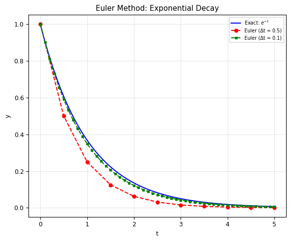
Error at t=5 (Δt=0.5): 0.0058
Error at t=5 (Δt=0.1): 0.0016
Ratio: 3.6x  (5x smaller Δt → ~5x smaller error)
Application: Falling with Air Drag#
A falling object with quadratic drag:
Terminal velocity: \(v_T = \sqrt{mg/b}\) when \(\dot{v} = 0\).
# Falling with quadratic drag
g = 9.81   # m/s^2
b_over_m = 0.1  # drag coefficient / mass
v_terminal = np.sqrt(g / b_over_m)

def falling_drag(t, y):
    """y = [height, velocity]. Positive v = downward."""
    h, v = y
    dhdt = -v           # height decreases as we fall
    dvdt = g - b_over_m * v**2  # gravity - drag
    return [dhdt, dvdt]

# Solve with Euler
t_fall, y_fall = euler(falling_drag, [0, 15], [1000, 0], dt=0.05)

fig, (ax1, ax2) = plt.subplots(2, 1, figsize=(6, 8))

ax1.plot(t_fall, y_fall[:, 1], 'b-', linewidth=1)
ax1.axhline(v_terminal, color='r', linestyle='--', label=f'Terminal velocity = {v_terminal:.1f} m/s')
ax1.set_xlabel('Time (s)')
ax1.set_ylabel('Velocity (m/s)')
ax1.set_title('Falling with Quadratic Drag')
ax1.legend(fontsize=7)
ax1.grid(True, alpha=0.3)

ax2.plot(t_fall, y_fall[:, 0], 'g-', linewidth=1)
ax2.set_xlabel('Time (s)')
ax2.set_ylabel('Height (m)')
ax2.set_title('Height vs Time')
ax2.grid(True, alpha=0.3)

plt.tight_layout()
plt.show()

print(f"Velocity approaches terminal velocity v_T = {v_terminal:.1f} m/s")
print(f"After ~5 time constants: v ≈ v_T")
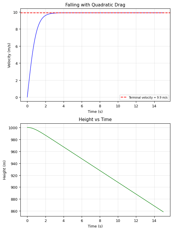
Velocity approaches terminal velocity v_T = 9.9 m/s
After ~5 time constants: v ≈ v_T
III. Euler Fails for Oscillators!#
The Simple Harmonic Oscillator#
Energy should be conserved: \(E = \frac{1}{2}v^2 + \frac{1}{2}\omega^2 x^2 = \text{const}\)
Let’s see what Euler does…
# Simple harmonic oscillator with Euler
omega = 2 * np.pi  # angular frequency (1 Hz)

def sho(t, y):
    """Simple harmonic oscillator: y = [x, v]."""
    x, v = y
    return [v, -omega**2 * x]

dt = 0.01
t_sho, y_sho = euler(sho, [0, 10], [1.0, 0.0], dt=dt)

# Exact solution
x_exact = np.cos(omega * t_sho)
energy = 0.5 * y_sho[:, 1]**2 + 0.5 * omega**2 * y_sho[:, 0]**2

fig, axes = plt.subplots(3, 1, figsize=(6, 10))

# Position
axes[0].plot(t_sho, x_exact, 'b-', linewidth=1, label='Exact', alpha=0.7)
axes[0].plot(t_sho, y_sho[:, 0], 'r-', linewidth=0.8, label='Euler')
axes[0].set_ylabel('x(t)')
axes[0].set_title(f'Euler Method on Harmonic Oscillator (Δt = {dt})')
axes[0].legend(fontsize=7)
axes[0].grid(True, alpha=0.3)

# Phase space
theta = np.linspace(0, 2*np.pi, 100)
axes[1].plot(np.cos(theta), -omega*np.sin(theta), 'b--', alpha=0.5, label='Exact (circle)')
axes[1].plot(y_sho[:, 0], y_sho[:, 1], 'r-', linewidth=0.5, label='Euler (spiral out!)')
axes[1].set_xlabel('x')
axes[1].set_ylabel('v')
axes[1].set_title('Phase Space')
axes[1].set_aspect('equal')
axes[1].legend(fontsize=7)
axes[1].grid(True, alpha=0.3)

# Energy
axes[2].plot(t_sho, energy / energy[0], 'r-', linewidth=0.8)
axes[2].axhline(1.0, color='b', linestyle='--', alpha=0.5, label='True energy (constant)')
axes[2].set_xlabel('t')
axes[2].set_ylabel('E(t) / E(0)')
axes[2].set_title('Energy — Euler adds energy over time!')
axes[2].legend(fontsize=7)
axes[2].grid(True, alpha=0.3)

plt.tight_layout()
plt.show()

print(f"Energy after 10 periods: {energy[-1]/energy[0]:.2f}x initial — Euler GAINS energy!")
print("The phase-space orbit spirals OUTWARD. This is unphysical.")
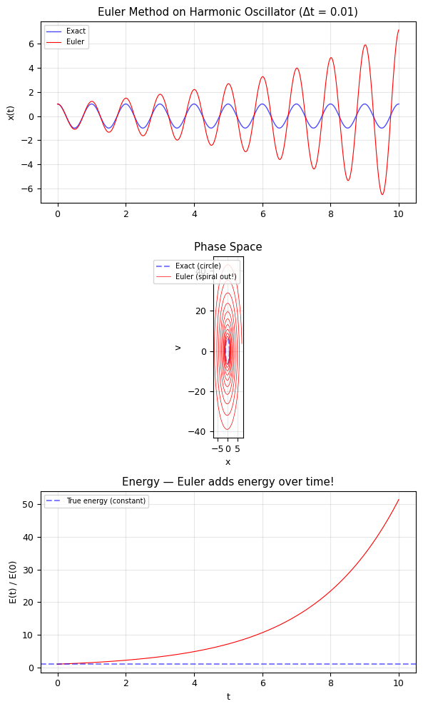
Energy after 10 periods: 51.42x initial — Euler GAINS energy!
The phase-space orbit spirals OUTWARD. This is unphysical.
The Problem#
Euler uses the old position to update both position and velocity simultaneously:
Both updates use data from time \(t_n\). For oscillators, this systematically adds energy at every step.
IV. The Euler-Cromer (Symplectic) Method#
Simple fix: update velocity first, then use the new velocity to update position:
This is a symplectic integrator — it preserves the geometric structure of Hamiltonian mechanics. Energy oscillates around the true value instead of drifting.
def euler_cromer(t_span, x0, v0, a_func, dt):
    """Solve x'' = a(x, v, t) using the Euler-Cromer (symplectic) method.

    Parameters
    ----------
    t_span : tuple
        (t_start, t_end).
    x0, v0 : float
        Initial position and velocity.
    a_func : callable
        Acceleration function a(x, v, t).
    dt : float
        Time step.

    Returns
    -------
    t, x, v : ndarrays
    """
    t = np.arange(t_span[0], t_span[1] + dt/2, dt)
    x = np.zeros(len(t))
    v = np.zeros(len(t))
    x[0], v[0] = x0, v0

    for i in range(len(t) - 1):
        v[i+1] = v[i] + dt * a_func(x[i], v[i], t[i])       # Update v FIRST
        x[i+1] = x[i] + dt * v[i+1]                  # Use NEW v

    return t, x, v

# Compare Euler vs Euler-Cromer on SHO
a_sho = lambda x, v, t: -omega**2 * x

t_ec, x_ec, v_ec = euler_cromer([0, 10], 1.0, 0.0, a_sho, dt=0.01)
energy_ec = 0.5 * v_ec**2 + 0.5 * omega**2 * x_ec**2

fig, (ax1, ax2) = plt.subplots(2, 1, figsize=(6, 8))

# Phase space comparison
ax1.plot(np.cos(theta), -omega*np.sin(theta), 'b--', alpha=0.5, linewidth=2, label='Exact')
ax1.plot(y_sho[:, 0], y_sho[:, 1], 'r-', linewidth=0.5, alpha=0.7, label='Euler (spirals out)')
ax1.plot(x_ec, v_ec, 'g-', linewidth=0.5, label='Euler-Cromer (stays close!)')
ax1.set_xlabel('x')
ax1.set_ylabel('v')
ax1.set_title('Phase Space: Euler vs Euler-Cromer')
ax1.set_aspect('equal')
ax1.legend(fontsize=7)
ax1.grid(True, alpha=0.3)

# Energy comparison
ax2.plot(t_sho, energy / energy[0], 'r-', linewidth=0.8, label='Euler (drifts up!)')
ax2.plot(t_ec, energy_ec / energy_ec[0], 'g-', linewidth=0.8, label='Euler-Cromer (bounded!)')
ax2.axhline(1.0, color='b', linestyle='--', alpha=0.5)
ax2.set_xlabel('t')
ax2.set_ylabel('E(t) / E(0)')
ax2.set_title('Energy Conservation')
ax2.legend(fontsize=7)
ax2.grid(True, alpha=0.3)

plt.tight_layout()
plt.show()

print(f"Euler energy drift after 10 periods: {energy[-1]/energy[0]:.4f}")
print(f"Euler-Cromer energy after 10 periods: {energy_ec[-1]/energy_ec[0]:.6f}")
print("\nEuler-Cromer oscillates around E=1 but never drifts — symplectic!")
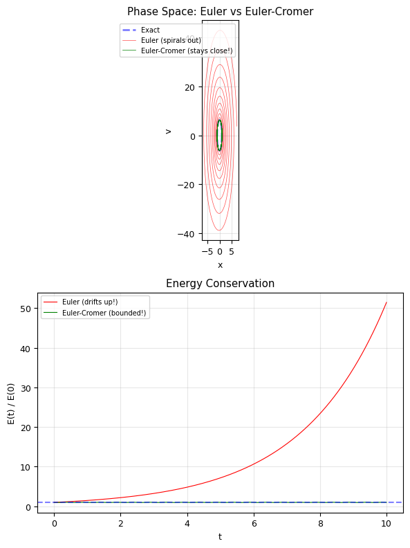
Euler energy drift after 10 periods: 51.4222
Euler-Cromer energy after 10 periods: 0.999350

Euler-Cromer oscillates around E=1 but never drifts — symplectic!
Why Symplectic Matters#
Method |
Energy behavior |
Best for |
|---|---|---|
Euler |
Drifts (grows) |
Short simulations, dissipative systems |
Euler-Cromer |
Bounded oscillation |
Long-time Hamiltonian dynamics |
Verlet / Leapfrog |
Bounded, 2nd order |
Molecular dynamics (we’ll see later) |
Molecular dynamics simulations of millions of atoms for nanoseconds require symplectic integrators.
V. The Runge-Kutta Method (RK4)#
Euler uses the slope at one point. RK4 samples the slope at four points per step:
Global error: \(O(\Delta t^4)\) — fourth-order method. 4× the work per step, but much more accurate.
def rk4(f, t_span, y0, dt):
    """Solve dy/dt = f(t, y) using the classic Runge-Kutta 4th order method.

    Parameters
    ----------
    f : callable
        Right-hand side f(t, y).
    t_span : tuple
        (t_start, t_end).
    y0 : array_like
        Initial condition.
    dt : float
        Time step.

    Returns
    -------
    t, y : ndarrays
    """
    t_start, t_end = t_span
    t = np.arange(t_start, t_end + dt/2, dt)
    y0 = np.atleast_1d(np.array(y0, dtype=float))
    y = np.zeros((len(t), len(y0)))
    y[0] = y0

    for i in range(len(t) - 1):
        k1 = np.array(f(t[i], y[i]))
        k2 = np.array(f(t[i] + dt/2, y[i] + dt/2 * k1))
        k3 = np.array(f(t[i] + dt/2, y[i] + dt/2 * k2))
        k4 = np.array(f(t[i] + dt, y[i] + dt * k3))
        y[i+1] = y[i] + dt/6 * (k1 + 2*k2 + 2*k3 + k4)

    return t, y

# Compare Euler vs RK4 on the SHO
dt_compare = 0.05  # Larger step to show the difference

t_e, y_e = euler(sho, [0, 2], [1.0, 0.0], dt=dt_compare)
t_r, y_r = rk4(sho, [0, 2], [1.0, 0.0], dt=dt_compare)
x_exact_c = np.cos(omega * t_e)

fig, (ax1, ax2) = plt.subplots(2, 1, figsize=(6, 8))

ax1.plot(t_e, x_exact_c, 'b-', linewidth=1.5, label='Exact', alpha=0.7)
ax1.plot(t_e, y_e[:, 0], 'r--', linewidth=0.8, label='Euler')
ax1.plot(t_r, y_r[:, 0], 'g-', linewidth=0.8, label='RK4')
ax1.set_ylabel('x(t)')
ax1.set_title(f'Euler vs RK4 (Δt = {dt_compare})')
ax1.legend(fontsize=7)
ax1.grid(True, alpha=0.3)

# Error comparison
err_euler = np.abs(y_e[:, 0] - np.cos(omega * t_e))
err_rk4 = np.abs(y_r[:, 0] - np.cos(omega * t_r))

ax2.semilogy(t_e, err_euler + 1e-16, 'r-', linewidth=0.8, label='Euler error')
ax2.semilogy(t_r, err_rk4 + 1e-16, 'g-', linewidth=0.8, label='RK4 error')
ax2.set_xlabel('t')
ax2.set_ylabel('|error|')
ax2.set_title('Error Comparison')
ax2.legend(fontsize=7)
ax2.grid(True, alpha=0.3)

plt.tight_layout()
plt.show()

print(f"Euler error at t=10: {err_euler[-1]:.4f}")
print(f"RK4 error at t=10:   {err_rk4[-1]:.2e}")
print(f"RK4 is ~{err_euler[-1]/max(err_rk4[-1], 1e-16):.0f}× more accurate with the same Δt!")
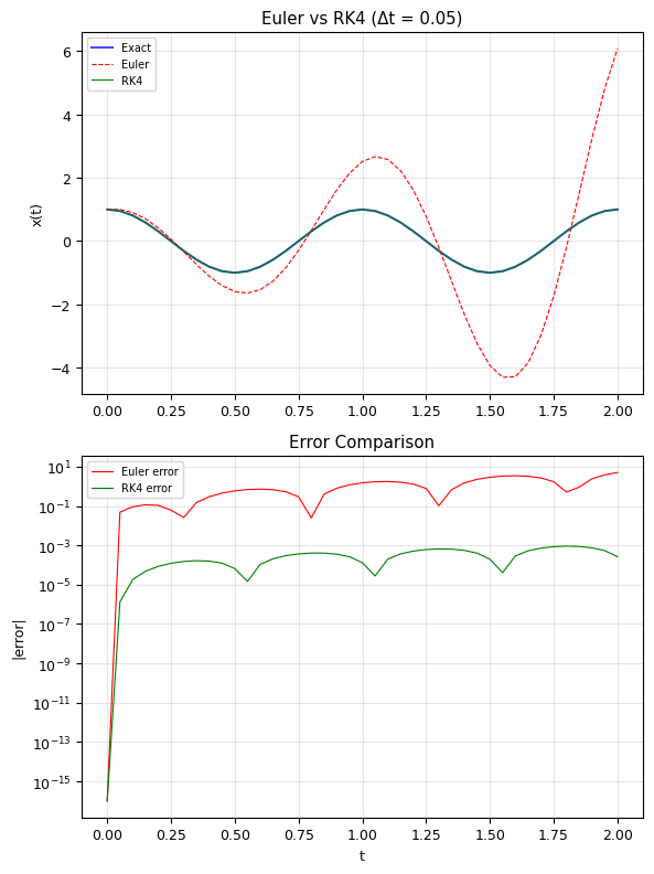
Euler error at t=10: 5.0751
RK4 error at t=10:   2.64e-04
RK4 is ~19209× more accurate with the same Δt!
Method Comparison Summary#
Method |
Order |
Error per step |
Evaluations per step |
Best for |
|---|---|---|---|---|
Euler |
1st |
\(O(\Delta t^2)\) |
1 |
Learning, simple problems |
Euler-Cromer |
1st |
\(O(\Delta t^2)\) |
1 |
Long-time Hamiltonian dynamics |
RK4 |
4th |
\(O(\Delta t^5)\) |
4 |
General-purpose ODE solving |
RK45 (adaptive) |
4th–5th |
Automatic |
6 |
Production code ( |
VI. The Professional Tool: scipy.integrate.solve_ivp#
In practice, we use scipy’s adaptive solver. It automatically:
Adjusts the step size for accuracy
Uses embedded error estimates (RK45: 4th and 5th order)
Handles stiff equations (with
method='Radau'or'BDF')
sol = solve_ivp(f, t_span, y0, t_eval=t_points, method='RK45')
## sol.t = time points
## sol.y = solution (shape: n_variables × n_timepoints)
# Damped harmonic oscillator with solve_ivp
# m*x'' + c*x' + k*x = 0  →  x'' = -(c/m)*v - (k/m)*x

def damped_oscillator(t, y, gamma, omega0):
    """Damped harmonic oscillator.

    Parameters
    ----------
    gamma : float
        Damping coefficient c/(2m).
    omega0 : float
        Natural frequency sqrt(k/m).
    """
    x, v = y
    return [v, -2*gamma*v - omega0**2 * x]

omega0 = 2 * np.pi  # natural frequency
t_eval = np.linspace(0, 5, 500)

# Three damping regimes
cases = {
    'Underdamped (ζ=0.1)': 0.1 * omega0,
    'Critically damped (ζ=1)': 1.0 * omega0,
    'Overdamped (ζ=2)': 2.0 * omega0
}

fig, (ax1, ax2) = plt.subplots(2, 1, figsize=(6, 8))

for label, gamma in cases.items():
    sol = solve_ivp(damped_oscillator, [0, 5], [1.0, 0.0],
                    t_eval=t_eval, args=(gamma, omega0))
    ax1.plot(sol.t, sol.y[0], linewidth=1, label=label)
    ax2.plot(sol.y[0], sol.y[1], linewidth=0.8, label=label)

ax1.set_xlabel('t (s)')
ax1.set_ylabel('x(t)')
ax1.set_title('Damped Harmonic Oscillator — Three Regimes')
ax1.axhline(0, color='k', linewidth=0.5)
ax1.legend(fontsize=7)
ax1.grid(True, alpha=0.3)

ax2.set_xlabel('x')
ax2.set_ylabel('v')
ax2.set_title('Phase Space')
ax2.legend(fontsize=7)
ax2.grid(True, alpha=0.3)

plt.tight_layout()
plt.show()

print("ζ < 1: Underdamped — oscillates with decaying envelope")
print("ζ = 1: Critically damped — fastest return to equilibrium without oscillation")
print("ζ > 1: Overdamped — slow return, no oscillation")
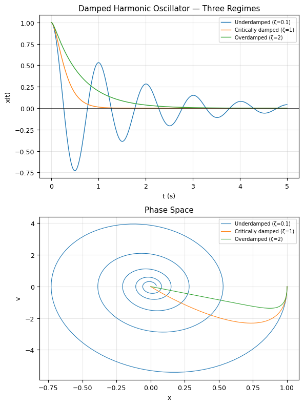
ζ < 1: Underdamped — oscillates with decaying envelope
ζ = 1: Critically damped — fastest return to equilibrium without oscillation
ζ > 1: Overdamped — slow return, no oscillation
VII. Physics Application: Phonons in a 1D Crystal#
The Monatomic Chain#
A chain of \(N\) atoms connected by springs (nearest-neighbor interaction):
where \(u_n\) is the displacement of atom \(n\) from equilibrium.
This is a system of \(N\) coupled ODEs — a perfect test for our methods!
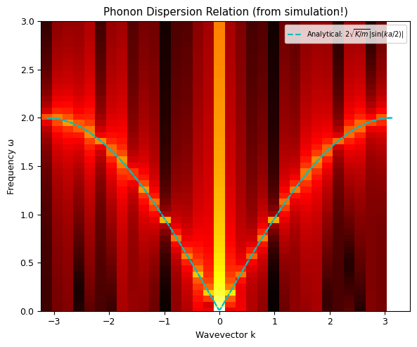
Analytical Dispersion Relation#
where \(a\) is the lattice spacing and \(k\) is the wavevector.
# 1D monatomic chain — phonon simulation
N_atoms = 32      # Number of atoms
K = 1.0           # Spring constant
m = 1.0           # Atom mass
a = 1.0           # Lattice spacing

def monatomic_chain(t, y):
    """Equations of motion for 1D monatomic chain.

    y = [u_0, u_1, ..., u_{N-1}, v_0, v_1, ..., v_{N-1}]
    Periodic boundary conditions.
    """
    u = y[:N_atoms]       # Displacements
    v = y[N_atoms:]       # Velocities

    # Acceleration: a_n = (K/m) * (u_{n+1} - 2*u_n + u_{n-1})
    # Periodic BC: u[-1] = u[N-1], u[N] = u[0]
    u_right = np.roll(u, -1)  # u_{n+1}
    u_left = np.roll(u, 1)    # u_{n-1}
    acc = (K / m) * (u_right - 2*u + u_left)

    return np.concatenate([v, acc])

# Initial condition: single atom displaced (impulse)
u0 = np.zeros(N_atoms)
u0[N_atoms // 2] = 1.0  # Displace the middle atom
v0 = np.zeros(N_atoms)
y0_chain = np.concatenate([u0, v0])

# Solve
T_sim = 40
t_eval_chain = np.linspace(0, T_sim, 500)
sol_chain = solve_ivp(monatomic_chain, [0, T_sim], y0_chain,
                       t_eval=t_eval_chain, method='RK45', rtol=1e-8)

# Extract displacements
U = sol_chain.y[:N_atoms, :]

# Plot as heatmap: atom index vs time
fig, ax = plt.subplots(figsize=(6, 5))
im = ax.pcolormesh(sol_chain.t, np.arange(N_atoms), U,
                    cmap='RdBu_r', shading='auto', vmin=-0.3, vmax=0.3)
plt.colorbar(im, ax=ax, label='Displacement $u_n$')
ax.set_xlabel('Time')
ax.set_ylabel('Atom index n')
ax.set_title('Phonon Propagation in 1D Crystal')
plt.tight_layout()
plt.show()

print("A single displaced atom → waves propagate outward in both directions!")
print("Periodic BC: waves wrap around and interfere.")
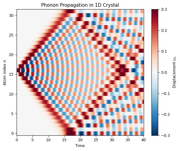
A single displaced atom → waves propagate outward in both directions!
Periodic BC: waves wrap around and interfere.
# Extract the dispersion relation from the simulation using 2D FFT!
# FFT in space → wavevector k
# FFT in time → frequency ω

# Use a longer, finer simulation for better resolution
T_long = 100
N_time = 2048
t_fine = np.linspace(0, T_long, N_time)

# Random initial displacements to excite all modes
np.random.seed(42)
u0_rand = 0.1 * np.random.randn(N_atoms)
v0_rand = 0.1 * np.random.randn(N_atoms)
y0_rand = np.concatenate([u0_rand, v0_rand])

sol_long = solve_ivp(monatomic_chain, [0, T_long], y0_rand,
                      t_eval=t_fine, method='RK45', rtol=1e-8)
U_long = sol_long.y[:N_atoms, :]

# 2D FFT: space-time → (k, ω)
F_2d = np.fft.fft2(U_long)
power = np.abs(np.fft.fftshift(F_2d))**2

# Frequency and wavevector axes
dk = 2 * np.pi / (N_atoms * a)
k_axis = np.fft.fftshift(np.fft.fftfreq(N_atoms, d=a)) * 2 * np.pi
dt_sim = T_long / N_time
omega_axis = np.fft.fftshift(np.fft.fftfreq(N_time, d=dt_sim)) * 2 * np.pi

# Analytical dispersion
k_theory = np.linspace(-np.pi/a, np.pi/a, 200)
omega_theory = 2 * np.sqrt(K/m) * np.abs(np.sin(k_theory * a / 2))

fig, ax = plt.subplots(figsize=(6, 5))
# Only show positive frequencies
omega_pos = omega_axis >= 0
ax.pcolormesh(k_axis, omega_axis[omega_pos],
              np.log10(power[:, omega_pos].T + 1),
              cmap='hot', shading='auto')

ax.plot(k_theory, omega_theory, 'c--', linewidth=1.5, label='Analytical: $2\sqrt{K/m}|\sin(ka/2)|$')
ax.plot(-k_theory, omega_theory, 'c--', linewidth=1.5)

ax.set_xlabel('Wavevector k')
ax.set_ylabel('Frequency ω')
ax.set_title('Phonon Dispersion Relation (from simulation!)')
ax.set_ylim(0, 3)
ax.legend(fontsize=7)
plt.tight_layout()
plt.show()

print("Bright bands = normal modes of the crystal.")
print("Cyan dashed = analytical dispersion relation.")
print("They match! We recovered the phonon spectrum from a simulation.")
<>:41: SyntaxWarning: invalid escape sequence '\s'
<>:41: SyntaxWarning: invalid escape sequence '\s'
/tmp/ipython-input-432/3103749938.py:41: SyntaxWarning: invalid escape sequence '\s'
  ax.plot(k_theory, omega_theory, 'c--', linewidth=1.5, label='Analytical: $2\sqrt{K/m}|\sin(ka/2)|$')
Bright bands = normal modes of the crystal.
Cyan dashed = analytical dispersion relation.
They match! We recovered the phonon spectrum from a simulation.
VIII. Physics Application: Diatomic Chain (Optical & Acoustic Phonons)#
A chain with two different atom masses (\(m_1\), \(m_2\)) alternating:
This creates two branches:
Acoustic branch (low ω): atoms move in phase
Optical branch (high ω): atoms move out of phase
Band gap between them: no propagating modes!
# Diatomic chain simulation
N_cells = 16         # Unit cells (total 32 atoms)
N_total = 2 * N_cells
m1 = 1.0             # Light atom
m2 = 3.0             # Heavy atom
K_di = 1.0

# Mass array: alternating m1, m2, m1, m2, ...
masses = np.zeros(N_total)
masses[0::2] = m1
masses[1::2] = m2

def diatomic_chain(t, y):
    """Equations of motion for 1D diatomic chain with periodic BC."""
    u = y[:N_total]
    v = y[N_total:]
    u_right = np.roll(u, -1)
    u_left = np.roll(u, 1)
    acc = (K_di / masses) * (u_right - 2*u + u_left)
    return np.concatenate([v, acc])

# Random initial conditions to excite all modes
np.random.seed(123)
u0_di = 0.1 * np.random.randn(N_total)
v0_di = 0.1 * np.random.randn(N_total)
y0_di = np.concatenate([u0_di, v0_di])

T_di = 200
N_time_di = 4096
t_di = np.linspace(0, T_di, N_time_di)
sol_di = solve_ivp(diatomic_chain, [0, T_di], y0_di,
                    t_eval=t_di, method='RK45', rtol=1e-8)
U_di = sol_di.y[:N_total, :]

# 2D FFT to get dispersion
F_di = np.fft.fft2(U_di)
power_di = np.abs(np.fft.fftshift(F_di))**2

k_di_axis = np.fft.fftshift(np.fft.fftfreq(N_total, d=a/2)) * 2 * np.pi
dt_di = T_di / N_time_di
omega_di_axis = np.fft.fftshift(np.fft.fftfreq(N_time_di, d=dt_di)) * 2 * np.pi

# Analytical dispersion for diatomic chain
k_th = np.linspace(0, np.pi / a, 200)
# ω² = K(1/m1 + 1/m2) ± K*sqrt((1/m1+1/m2)² - 4sin²(ka/2)/(m1*m2))
sum_inv = 1/m1 + 1/m2
omega_sq_plus = K_di * (sum_inv + np.sqrt(sum_inv**2 - 4*np.sin(k_th*a/2)**2/(m1*m2)))
omega_sq_minus = K_di * (sum_inv - np.sqrt(sum_inv**2 - 4*np.sin(k_th*a/2)**2/(m1*m2)))
omega_optical = np.sqrt(omega_sq_plus)
omega_acoustic = np.sqrt(omega_sq_minus)

fig, ax = plt.subplots(figsize=(6, 5))
omega_pos_di = omega_di_axis >= 0
ax.pcolormesh(k_di_axis, omega_di_axis[omega_pos_di],
              np.log10(power_di[:, omega_pos_di].T + 1),
              cmap='hot', shading='auto')

ax.plot(k_th, omega_acoustic, 'c-', linewidth=1.5, label='Acoustic branch')
ax.plot(-k_th, omega_acoustic, 'c-', linewidth=1.5)
ax.plot(k_th, omega_optical, 'lime', linewidth=1.5, label='Optical branch')
ax.plot(-k_th, omega_optical, 'lime', linewidth=1.5)

# Band gap
omega_gap_low = np.sqrt(2*K_di/m2)
omega_gap_high = np.sqrt(2*K_di/m1)
ax.axhspan(omega_gap_low, omega_gap_high, alpha=0.15, color='yellow', label='Band gap')

ax.set_xlabel('Wavevector k')
ax.set_ylabel('Frequency ω')
ax.set_title(f'Diatomic Chain: Acoustic + Optical Phonons (m₂/m₁ = {m2/m1:.0f})')
ax.set_ylim(0, 2.0)
ax.legend(fontsize=7, loc='upper right')
plt.tight_layout()
plt.show()

print(f"Band gap: ω = {omega_gap_low:.3f} to {omega_gap_high:.3f}")
print(f"No propagating modes in the gap — this is why some crystals are transparent!")
print(f"The mass ratio m2/m1 = {m2/m1:.0f} controls the gap width.")
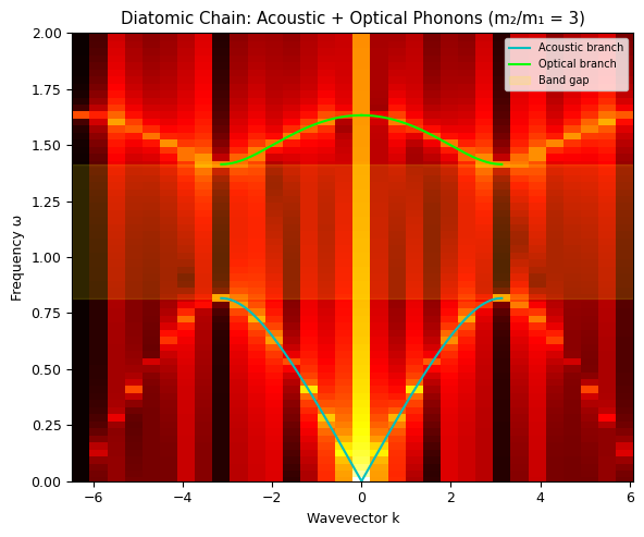
Band gap: ω = 0.816 to 1.414
No propagating modes in the gap — this is why some crystals are transparent!
The mass ratio m2/m1 = 3 controls the gap width.
IX. Physics Application: Nonlinear Pendulum#
The full pendulum equation (not the small-angle approximation):
For small \(\theta\): \(\sin\theta \approx \theta\) → SHO. For large \(\theta\): the period depends on amplitude!
# Nonlinear pendulum: compare small-angle vs full equation
g_pend = 9.81
L_pend = 1.0

def pendulum_full(t, y):
    theta, omega_p = y
    return [omega_p, -(g_pend/L_pend) * np.sin(theta)]

def pendulum_linear(t, y):
    theta, omega_p = y
    return [omega_p, -(g_pend/L_pend) * theta]

t_pend = np.linspace(0, 10, 1000)

fig, axes = plt.subplots(2, 1, figsize=(6, 8))

# Small angle: linear ≈ nonlinear
theta0_small = 0.1  # ~6°
sol_full_s = solve_ivp(pendulum_full, [0, 10], [theta0_small, 0], t_eval=t_pend)
sol_lin_s = solve_ivp(pendulum_linear, [0, 10], [theta0_small, 0], t_eval=t_pend)

axes[0].plot(sol_full_s.t, np.degrees(sol_full_s.y[0]), 'b-', label='Full (sin θ)')
axes[0].plot(sol_lin_s.t, np.degrees(sol_lin_s.y[0]), 'r--', label='Linear (θ)')
axes[0].set_title(f'Small angle: θ₀ = {np.degrees(theta0_small):.0f}° — linear works!')
axes[0].set_ylabel('θ (degrees)')
axes[0].legend(fontsize=7)
axes[0].grid(True, alpha=0.3)

# Large angle: linear fails
theta0_large = 2.5  # ~143°
sol_full_l = solve_ivp(pendulum_full, [0, 10], [theta0_large, 0], t_eval=t_pend)
sol_lin_l = solve_ivp(pendulum_linear, [0, 10], [theta0_large, 0], t_eval=t_pend)

axes[1].plot(sol_full_l.t, np.degrees(sol_full_l.y[0]), 'b-', label='Full (sin θ)')
axes[1].plot(sol_lin_l.t, np.degrees(sol_lin_l.y[0]), 'r--', label='Linear (θ)')
axes[1].set_title(f'Large angle: θ₀ = {np.degrees(theta0_large):.0f}° — linear fails!')
axes[1].set_xlabel('Time (s)')
axes[1].set_ylabel('θ (degrees)')
axes[1].legend(fontsize=7)
axes[1].grid(True, alpha=0.3)

plt.tight_layout()
plt.show()

# Measure periods
# Find zero-crossings of the full solution
from scipy.signal import find_peaks
peaks, _ = find_peaks(sol_full_l.y[0])
if len(peaks) >= 2:
    T_numerical = np.mean(np.diff(sol_full_l.t[peaks]))
    T_linear = 2 * np.pi * np.sqrt(L_pend / g_pend)
    print(f"\nLinear period:    T₀ = {T_linear:.4f} s")
    print(f"Nonlinear period: T  = {T_numerical:.4f} s  (θ₀ = {np.degrees(theta0_large):.0f}°)")
    print(f"Difference: {(T_numerical - T_linear)/T_linear * 100:.1f}% longer")
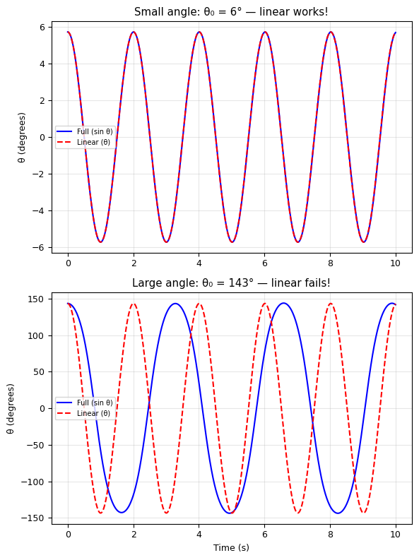
Linear period:    T₀ = 2.0061 s
Nonlinear period: T  = 3.3033 s  (θ₀ = 143°)
Difference: 64.7% longer