Numerical Integration#
Why Numerical Integration?#
Many integrals in physics cannot be solved analytically:
The integrand has no closed-form antiderivative
The function is defined by data points, not a formula
The integral is too complex for symbolic computation
import numpy as np
import matplotlib.pyplot as plt
from scipy import integrate

# For nicer plots
plt.rcParams['figure.figsize'] = [10, 6]
plt.rcParams['font.size'] = 12
I. The Integration Problem#
We want to compute the definite integral:
Geometrically, this is the signed area under the curve \(f(x)\) between \(x = a\) and \(x = b\).
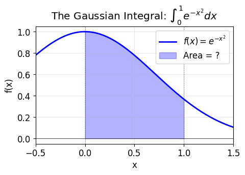
Example: An “Impossible” Integral#
Consider the Gaussian integral:
This integral has no closed-form antiderivative in terms of elementary functions! But we can compute it numerically.
# Visualize the integral we want to compute
def f(x):
    return np.exp(-x**2)

# f = lambda x: x**2

x = np.linspace(-0.5, 1.5, 200)
y = f(x)

# Area to integrate
x_fill = np.linspace(0, 1, 100)
y_fill = f(x_fill)

plt.figure(figsize=(5, 3))
plt.plot(x, y, 'b-', linewidth=2, label=r'$f(x) = e^{-x^2}$')
plt.fill_between(x_fill, y_fill, alpha=0.3, color='blue', label='Area = ?')
plt.axhline(y=0, color='k', linestyle='-', linewidth=0.5)
plt.axvline(x=0, color='k', linestyle='--', linewidth=0.5, alpha=0.5)
plt.axvline(x=1, color='k', linestyle='--', linewidth=0.5, alpha=0.5)
plt.xlabel('x')
plt.ylabel('f(x)')
plt.title(r'The Gaussian Integral: $\int_0^1 e^{-x^2} dx$')
plt.legend()
plt.grid(True, alpha=0.3)
plt.xlim(-0.5, 1.5)
plt.show()
II. Riemann Sums#
The fundamental idea: approximate the area with rectangles.
Divide \([a, b]\) into \(n\) subintervals of width \(h = \frac{b-a}{n}\)
Approximate the area in each subinterval with a rectangle
Sum all the rectangles
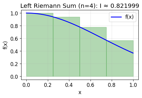
Left Riemann Sum#
Use the left endpoint of each subinterval:
where \(x_i = a + i \cdot h\)
def visualize_riemann(f, a, b, n, method='left'):
"""Visualize Riemann sum approximation."""
h = (b - a) / n
x_fine = np.linspace(a, b, 200)
plt.figure(figsize=(5, 3))
plt.plot(x_fine, f(x_fine), 'b-', linewidth=2, label='f(x)')
total = 0
for i in range(n):
x_left = a + i * h
x_right = x_left + h
if method == 'left':
height = f(x_left)
elif method == 'right':
height = f(x_right)
elif method == 'midpoint':
height = f((x_left + x_right) / 2)
total += height * h
# Draw rectangle
rect = plt.Rectangle((x_left, 0), h, height,
fill=True, alpha=0.3, color='green',
edgecolor='green', linewidth=1)
plt.gca().add_patch(rect)
plt.xlabel('x')
plt.ylabel('f(x)')
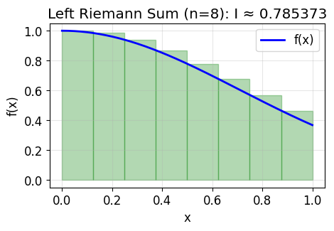
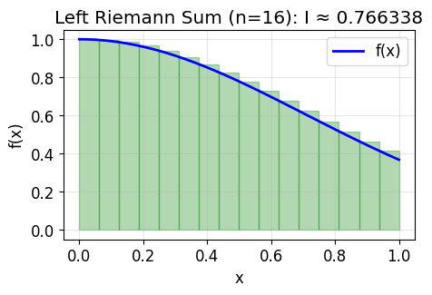
plt.title(f'{method.capitalize()} Riemann Sum (n={n}): I ≈ {total:.6f}')
plt.legend()
plt.grid(True, alpha=0.3)
plt.show()
return total
# Visualize left Riemann sum with different n values
print("Left Riemann Sum:")
for n in [4, 8, 16]:
result = visualize_riemann(f, 0, 1, n, 'left')
Left Riemann Sum:
/tmp/ipython-input-1523402423.py:24: UserWarning: Setting the 'color' property will override the edgecolor or facecolor properties.
  rect = plt.Rectangle((x_left, 0), h, height,
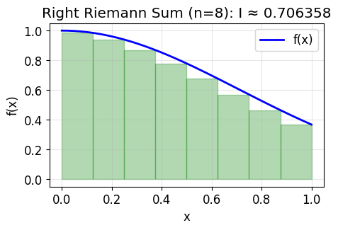
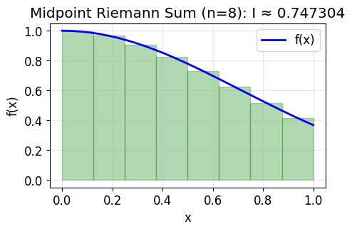
Right and Midpoint Riemann Sums#
Right Riemann Sum: Use the right endpoint $\(I \approx \sum_{i=1}^{n} f(x_i) \cdot h\)$
Midpoint Rule: Use the midpoint (often more accurate!) $\(I \approx \sum_{i=0}^{n-1} f\left(x_i + \frac{h}{2}\right) \cdot h\)$
# Compare different Riemann sums
print("Comparison of Riemann Sum Methods (n=8):")
print("=" * 40)

for method in ['left', 'right', 'midpoint']:
    result = visualize_riemann(f, 0, 1, 8, method)
Comparison of Riemann Sum Methods (n=8):
========================================
/tmp/ipython-input-1523402423.py:24: UserWarning: Setting the 'color' property will override the edgecolor or facecolor properties.
  rect = plt.Rectangle((x_left, 0), h, height,
Implementing Riemann Sums#
def riemann_sum(f, a, b, n, method='midpoint'):
    """
    Compute Riemann sum approximation of integral.

    Parameters:
        f: function to integrate
        a, b: integration limits
        n: number of subintervals
        method: 'left', 'right', or 'midpoint'

    Returns:
        Approximate value of the integral
    """
    h = (b - a) / n

    if method == 'left':
        x = np.linspace(a, b - h, n)
    elif method == 'right':
        x = np.linspace(a + h, b, n)
    elif method == 'midpoint':
        x = np.linspace(a + h/2, b - h/2, n)

    return np.sum(f(x)) * h

# Test with increasing n
print("Convergence of Midpoint Rule:")
print(f"{'n':>8} {'Integral':>15} {'Error':>15}")
print("-" * 40)

# True value (from scipy)
true_value, _ = integrate.quad(f, 0, 1)
# true_value = 1/3  # For f(x) = x^2 from 0 to 1

for n in [10, 100, 1000, 10000]:
    result = riemann_sum(f, 0, 1, n, 'midpoint')
    error = abs(result - true_value)
    print(f"{n:>8} {result:>15.10f} {error:>15.2e}")

print(f"\nTrue value: {true_value:.10f}")
Convergence of Midpoint Rule:
       n        Integral           Error
----------------------------------------
      10    0.7471308777        3.07e-04
     100    0.7468271985        3.07e-06
    1000    0.7468241635        3.07e-08
   10000    0.7468241331        3.07e-10

True value: 0.7468241328
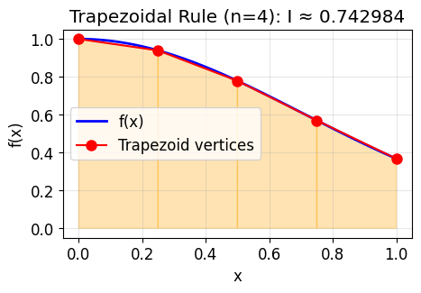
III. Trapezoidal Rule#
Instead of rectangles, use trapezoids to better approximate the curve.
For each subinterval, connect the endpoints with a straight line:
Or equivalently:
The trapezoidal rule is exact for linear functions and has error \(O(h^2)\).
def visualize_trapezoid(f, a, b, n):
    """Visualize trapezoidal rule approximation."""
    h = (b - a) / n
    x_points = np.linspace(a, b, n + 1)
    y_points = f(x_points)

    x_fine = np.linspace(a, b, 200)

    plt.figure(figsize=(5, 3))
    plt.plot(x_fine, f(x_fine), 'b-', linewidth=2, label='f(x)')

    # Draw trapezoids
    for i in range(n):
        x_trap = [x_points[i], x_points[i], x_points[i+1], x_points[i+1]]
        y_trap = [0, y_points[i], y_points[i+1], 0]
        plt.fill(x_trap, y_trap, alpha=0.3, color='orange', edgecolor='orange', linewidth=1)

    # Plot the approximating line segments
    plt.plot(x_points, y_points, 'ro-', markersize=8, label='Trapezoid vertices')

    # Compute integral
    integral = h * (0.5 * y_points[0] + np.sum(y_points[1:-1]) + 0.5 * y_points[-1])

    plt.xlabel('x')
    plt.ylabel('f(x)')
    plt.title(f'Trapezoidal Rule (n={n}): I ≈ {integral:.6f}')
    plt.legend()
    plt.grid(True, alpha=0.3)
    plt.show()

    return integral

# Visualize
for n in [4, 8]:
    result = visualize_trapezoid(f, 0, 1, n)

Implementing the Trapezoidal Rule#
def trapezoidal(f, a, b, n):
    """
    Compute integral using the trapezoidal rule.

    Parameters:
        f: function to integrate
        a, b: integration limits
        n: number of subintervals

    Returns:
        Approximate value of the integral
    """
    h = (b-a)/n
    x = np.linspace(a, b, n+1)
    y = f(x)

    # Trapezoidal formula
    return h * (y[0]*0.5 + y[-1]*0.5 + np.sum(y[1:-1]))

# Test convergence
print("Convergence of Trapezoidal Rule:")
print(f"{'n':>8} {'Integral':>15} {'Error':>15}")
print("-" * 40)

for n in [10, 100, 1000, 10000]:
    result = trapezoidal(f, 0, 1, n)
    error = abs(result - true_value)
    print(f"{n:>8} {result:>15.10f} {error:>15.2e}")

print(f"\nTrue value: {true_value:.10f}")
Convergence of Trapezoidal Rule:
       n        Integral           Error
----------------------------------------
      10    0.7462107961        6.13e-04
     100    0.7468180015        6.13e-06
    1000    0.7468240715        6.13e-08
   10000    0.7468241322        6.13e-10

True value: 0.7468241328
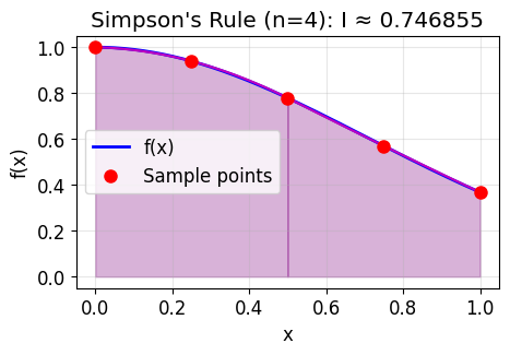
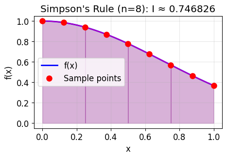
IV. Simpson’s Rule#
The trapezoidal rule is simple, taking only a few lines of code as we have seen. And it is often perfectly adequate for calculations where no great accuracy is required. It happens frequently in physics calculations that we don’t need an answer accurate to many significant figures and in such cases the ease and simplicity of the trapezoidal rule can make it the method of choice.
However, there are also cases where greater accuracy is required.
As we have seen we can increase the accuracy of the trapezoidal rule by increasing the number N of steps used in the calculation.
But in some cases, the calculation can become slow.
There are other, more advanced schemes for calculating integrals that can achieve high accuracy while still arriving at an answer quickly.
We can often get a better result if we approximate the function instead with curves of some kind.
Simpson’s rule does exactly this, using quadratic curves.
In order to specify a quadratic completely
one needs three points, not just two as with a straight line.
Suppose, as before, that our integrand is denoted f(x) and the spacing of adjacent points is \(h\). And suppose for the purposes of argument that we have three points at \(x\) = −h, 0, and +h. If we fit a quadratic \(Ax^2 + Bx + C\) through these points, then by definition we will have:
Solving these equations gives
and the area under the curve of f(x) from −h to +h is given approximately by the area under the quadratic:
This is Simpson’s rule. It gives us an approximation to the area under two adjacent slices of our function. Note that the final formula for the area involves only h and the value of the function at evenly spaced points, just as with the trapezoidal rule. So to use Simpson’s rule we don’t actually have to worry about the details of fitting a quadratic—we just plug numbers into this formula and it gives us an answer.
Applying Simpson’s rule involves dividing the domain of integration into many slices and using the rule to separately estimate the area under successive pairs of slices, then adding the estimates for all pairs to get the final answer. If, as before, we are integrating from \(x\) = a to \(x\) = b in slices of width \(h\) then the three points bounding the first pair of slices fall at \(x = a, a + h, a + 2h\), those bounding the second pair at \(a + 2h, a + 3h, a + 4h\), and so forth. Then the approximate value of the entire integral is given by
1/3 h (1, 4, 2,4,2,4,2,4….,4,1 )
see more details in: https://en.wikipedia.org/wiki/Simpson’s_rule
Simpson’s rule is exact for polynomials up to degree 3 and has error \(O(h^4)\) — much better than trapezoidal!
def visualize_simpson(f, a, b, n):
    """Visualize Simpson's rule with parabolas."""
    if n % 2 != 0:
        n += 1  # Ensure even

    h = (b - a) / n
    x_points = np.linspace(a, b, n + 1)
    y_points = f(x_points)

    x_fine = np.linspace(a, b, 200)

    plt.figure(figsize=(5, 3))
    plt.plot(x_fine, f(x_fine), 'b-', linewidth=2, label='f(x)')

    # Draw parabolic segments
    for i in range(0, n, 2):
        # Fit parabola through 3 points
        x3 = x_points[i:i+3]
        y3 = y_points[i:i+3]
        coeffs = np.polyfit(x3, y3, 2)

        x_para = np.linspace(x3[0], x3[2], 50)
        y_para = np.polyval(coeffs, x_para)

        plt.fill_between(x_para, y_para, alpha=0.3, color='purple')
        plt.plot(x_para, y_para, 'm-', linewidth=1.5)

    plt.plot(x_points, y_points, 'ro', markersize=8, label='Sample points')

    # Compute integral using Simpson's rule
    coefficients = np.ones(n + 1)
    coefficients[1:-1:2] = 4  # Odd indices
    coefficients[2:-1:2] = 2  # Even indices (except first and last)
    integral = h / 3 * np.sum(coefficients * y_points)

    plt.xlabel('x')
    plt.ylabel('f(x)')
    plt.title(f"Simpson's Rule (n={n}): I ≈ {integral:.6f}")
    plt.legend()
    plt.grid(True, alpha=0.3)
    plt.show()

    return integral

# Visualize
for n in [4, 8]:
    result = visualize_simpson(f, 0, 1, n)
Implementing Simpson’s Rule#
def simpson(f, a, b, n):
    """
    Compute integral using Simpson's rule.

    Parameters:
        f: function to integrate
        a, b: integration limits
        n: number of subintervals (must be even)

    Returns:
        Approximate value of the integral
    """
    if n % 2 != 0:
        raise ValueError("n must be even for Simpson's rule")

    h = (b - a) / n
    x = np.linspace(a, b, n + 1)
    y = f(x)

    # Simpson's coefficients: 1, 4, 2, 4, 2, ..., 4, 1
    coefficients = np.ones(n + 1)
    coefficients[1:-1:2] = 4
    coefficients[2:-1:2] = 2

    return  np.sum(coefficients * y) * h/3

# Test convergence
print("Convergence of Simpson's Rule:")
print(f"{'n':>8} {'Integral':>15} {'Error':>15}")
print("-" * 40)

for n in [10, 100, 1000, 10000]:
    result = simpson(f, 0, 1, n)
    error = abs(result - true_value)
    print(f"{n:>8} {result:>15.10f} {error:>15.2e}")

print(f"\nTrue value: {true_value:.10f}")
Convergence of Simpson's Rule:
       n        Integral           Error
----------------------------------------
      10    0.7468249483        8.15e-07
     100    0.7468241329        8.17e-11
    1000    0.7468241328        7.99e-15
   10000    0.7468241328        0.00e+00

True value: 0.7468241328
V. Using SciPy for Integration#
In practice, use scipy.integrate — it provides robust, well-tested implementations.
Main Functions#
Function |
Use Case |
|---|---|
|
General-purpose adaptive integration |
|
Trapezoidal rule for sampled data |
|
Simpson’s rule for sampled data |
|
Double integrals |
|
Triple integrals |
# scipy.integrate.quad - Adaptive quadrature
from scipy.integrate import quad

def f(x):
    return np.exp(-x**2)

# quad returns (value, error_estimate)
result, error = quad(f, 0, 1)

print("Using scipy.integrate.quad:")
print(f"  Integral: {result:.15f}")
print(f"  Error estimate: {error:.2e}")

# It can handle infinite limits!
result_inf, error_inf = quad(f, 0, np.inf)
print(f"\n∫₀^∞ e^(-x²) dx = {result_inf:.10f}")
print(f"(Exact: √π/2 = {np.sqrt(np.pi)/2:.10f})")
Using scipy.integrate.quad:
  Integral: 0.746824132812427
  Error estimate: 8.29e-15

∫₀^∞ e^(-x²) dx = 0.8862269255
(Exact: √π/2 = 0.8862269255)
Integrating Sampled Data#
When you have data points (not a function), use trapezoid() or simpson():
from scipy.integrate import trapezoid, simpson

# Sampled data (e.g., from an experiment)
x_data = np.array([0, 0.25, 0.5, 0.75, 1.0])
y_data = np.exp(-x_data**2)  # Simulating measured values

# Integrate using trapezoidal rule
result_trapz = trapezoid(y_data, x_data)

# Integrate using Simpson's rule
result_simp = simpson(y_data, x=x_data)

print("Integrating sampled data:")
print(f"  x = {x_data}")
print(f"  y = {np.round(y_data, 4)}")
print(f"\n  Trapezoidal: {result_trapz:.6f}")
print(f"  Simpson's:   {result_simp:.6f}")
print(f"  True value:  {true_value:.6f}")
Integrating sampled data:
  x = [0.   0.25 0.5  0.75 1.  ]
  y = [1.     0.9394 0.7788 0.5698 0.3679]

  Trapezoidal: 0.742984
  Simpson's:   0.746855
  True value:  0.746824
Multiple Integrals#
from scipy.integrate import dblquad

# Double integral: ∫∫ x*y dA over the unit square [0,1] × [0,1]
def integrand(y, x):  # Note: y first, then x!
    return x * y

result, error = dblquad(integrand, 0, 1, 0, 1)
print(f"∫∫ xy dA over [0,1]×[0,1] = {result:.6f}")
print(f"Exact: 1/4 = {0.25:.6f}")

# Volume of a hemisphere: ∫∫ √(R² - x² - y²) dA over disk of radius R
R = 1

def hemisphere(y, x):
    r2 = x**2 + y**2
    if r2 < R**2:
        return np.sqrt(R**2 - r2)
    return 0

def y_lower(x):
    return -np.sqrt(max(0, R**2 - x**2))

def y_upper(x):
    return np.sqrt(max(0, R**2 - x**2))

volume, _ = dblquad(hemisphere, -R, R, y_lower, y_upper)
print(f"\nVolume of hemisphere (R=1): {volume:.6f}")
print(f"Exact: (2/3)πR³ = {2/3 * np.pi * R**3:.6f}")
∫∫ xy dA over [0,1]×[0,1] = 0.250000
Exact: 1/4 = 0.250000

Volume of hemisphere (R=1): 2.094395
Exact: (2/3)πR³ = 2.094395
VI. Physics Applications#
Let’s apply numerical integration to real physics problems!
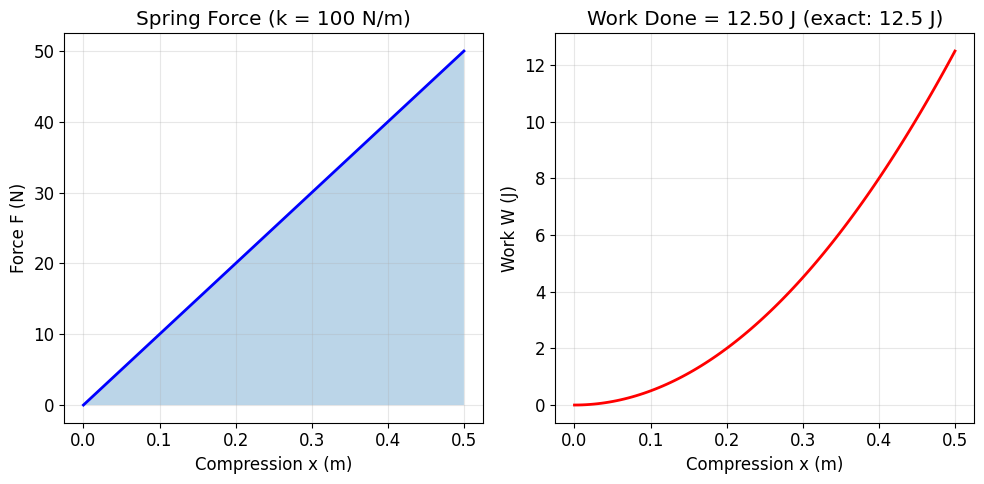
1. Work Done by a Variable Force#
The work done by a force \(F(x)\) moving an object from \(a\) to \(b\):
# Work to compress a spring (Hooke's Law: F = kx)
k = 100  # N/m (spring constant)

def spring_force(x):
    return k * x

# Compress spring from 0 to 0.5 meters
x = np.linspace(0, 0.5, 100)
F = spring_force(x)

# Compute work
W, _ = quad(spring_force, 0, 0.5)

# Exact: W = (1/2)kx² = 0.5 * 100 * 0.5² = 12.5 J

plt.figure(figsize=(10, 5))
plt.subplot(1, 2, 1)
plt.plot(x, F, 'b-', linewidth=2)
plt.fill_between(x, F, alpha=0.3)
plt.xlabel('Compression x (m)')
plt.ylabel('Force F (N)')
plt.title(f'Spring Force (k = {k} N/m)')
plt.grid(True, alpha=0.3)

plt.subplot(1, 2, 2)
# Cumulative work as function of compression
W_cumulative = [quad(spring_force, 0, xi)[0] for xi in x]
plt.plot(x, W_cumulative, 'r-', linewidth=2)
plt.xlabel('Compression x (m)')
plt.ylabel('Work W (J)')
plt.title(f'Work Done = {W:.2f} J (exact: 12.5 J)')
plt.grid(True, alpha=0.3)

plt.tight_layout()
plt.show()
2. Center of Mass of a Non-Uniform Rod#
For a rod with linear density \(\lambda(x)\):
# Rod with linearly increasing density: λ(x) = λ₀(1 + x/L)
L = 1.0  # Length of rod (m)
lambda0 = 2.0  # kg/m at x=0

def density(x):
    return lambda0 * (1 + x / L)

def x_times_density(x):
    return x * density(x)

# Total mass
M, _ = quad(density, 0, L)

# First moment
moment, _ = quad(x_times_density, 0, L)

# Center of mass
x_cm = moment / M

# Visualize
x = np.linspace(0, L, 100)

plt.figure(figsize=(10, 5))
plt.subplot(1, 2, 1)
plt.plot(x, density(x), 'b-', linewidth=2)
plt.fill_between(x, density(x), alpha=0.3)
plt.xlabel('Position x (m)')
plt.ylabel('Linear density λ (kg/m)')
plt.title('Non-uniform Rod Density')
plt.grid(True, alpha=0.3)

plt.subplot(1, 2, 2)
# Show rod as colored bar
for i in range(50):
    xi = i * L / 50
    color_intensity = density(xi) / density(L)
    plt.barh(0, L/50, left=xi, height=0.2, color=plt.cm.Blues(color_intensity))
plt.axvline(x_cm, color='red', linewidth=2, linestyle='--', label=f'Center of mass = {x_cm:.3f} m')
plt.axvline(L/2, color='green', linewidth=2, linestyle=':', label='Geometric center = 0.5 m')
plt.xlabel('Position x (m)')
plt.xlim(-0.1, 1.1)
plt.ylim(-0.5, 0.5)
plt.legend()
plt.title(f'Center of Mass (M = {M:.2f} kg)')
plt.grid(True, alpha=0.3)

plt.tight_layout()
plt.show()

print(f"Total mass: M = {M:.4f} kg")
print(f"Center of mass: x_cm = {x_cm:.4f} m")
print(f"(The heavier end pulls the center of mass toward x = L)")
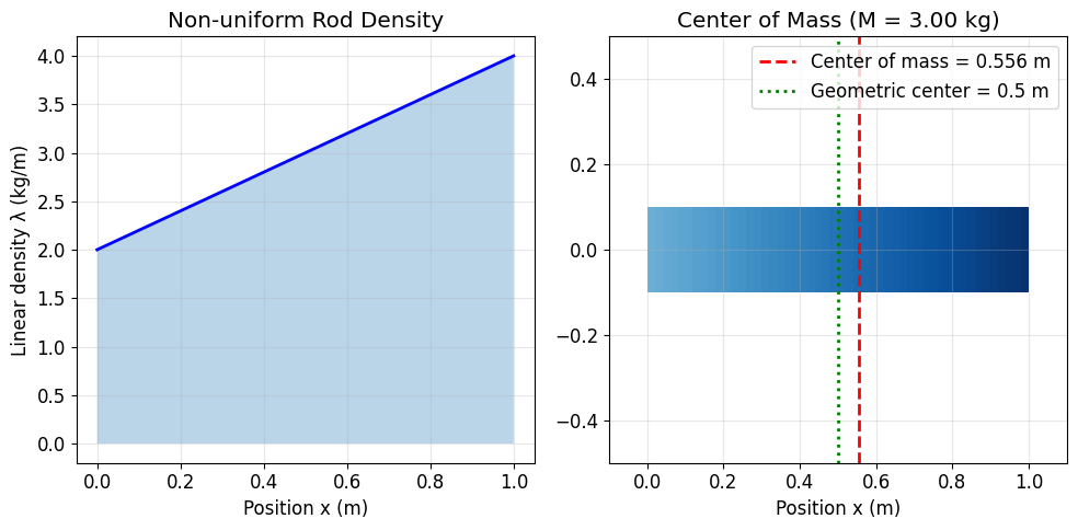
Total mass: M = 3.0000 kg
Center of mass: x_cm = 0.5556 m
(The heavier end pulls the center of mass toward x = L)
3. Probability from a Distribution#
For a probability density function \(p(x)\), the probability of \(x\) being in \([a, b]\):
# Maxwell-Boltzmann speed distribution
# p(v) = 4π(m/2πkT)^(3/2) * v² * exp(-mv²/2kT)

def maxwell_boltzmann(v, T, m):
    """Maxwell-Boltzmann speed distribution."""
    kB = 1.38e-23  # Boltzmann constant
    a = m / (2 * kB * T)
    return 4 * np.pi * (a / np.pi)**(3/2) * v**2 * np.exp(-a * v**2)

# Nitrogen molecule at room temperature
m_N2 = 28 * 1.66e-27  # kg (N₂ mass)
T = 300  # K

v = np.linspace(0, 1500, 500)  # m/s
p = maxwell_boltzmann(v, T, m_N2)

# Probability that speed is between 400 and 600 m/s
prob, _ = quad(lambda v: maxwell_boltzmann(v, T, m_N2), 400, 600)

# Most probable speed
v_mp = np.sqrt(2 * 1.38e-23 * T / m_N2)

# Mean speed
mean_v, _ = quad(lambda v: v * maxwell_boltzmann(v, T, m_N2), 0, 3000)

plt.figure(figsize=(5, 3))
plt.plot(v, p, 'b-', linewidth=2, label='Maxwell-Boltzmann distribution')
plt.fill_between(v[(v >= 400) & (v <= 600)],
                 p[(v >= 400) & (v <= 600)],
                 alpha=0.3, color='red',
                 label=f'P(400 < v < 600) = {prob:.3f}')
plt.axvline(v_mp, color='green', linestyle='--', label=f'Most probable: {v_mp:.0f} m/s')
plt.axvline(mean_v, color='orange', linestyle=':', label=f'Mean: {mean_v:.0f} m/s')

plt.xlabel('Speed v (m/s)')
plt.ylabel('Probability density p(v)')
plt.title(f'Maxwell-Boltzmann Distribution (N₂ at T = {T} K)')
plt.legend()
plt.grid(True, alpha=0.3)
plt.show()

print(f"Probability that N₂ molecule has speed between 400-600 m/s: {prob*100:.1f}%")
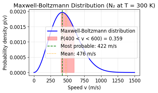
Probability that N₂ molecule has speed between 400-600 m/s: 35.9%
VII. Summary#
Methods Learned#
Method |
Order |
Best For |
|---|---|---|
Riemann Sum |
\(O(h)\) or \(O(h^2)\) |
Understanding the concept |
Trapezoidal |
\(O(h^2)\) |
Quick calculations, sampled data |
Simpson’s |
\(O(h^4)\) |
Smooth functions, high accuracy |
|
Adaptive |
Production code |
Key Takeaways#
Higher-order methods converge faster — Simpson’s needs far fewer points than trapezoidal for the same accuracy
Use SciPy in practice —
quad()handles edge cases and adapts automaticallyFor sampled data, use
trapezoid()orsimpson()from scipyCheck convergence — increase n and verify the result doesn’t change significantly
Coming Up Next#
Numerical Differentiation — computing derivatives from functions or data