Lecture 14: Monte Carlo Methods II — MCMC & Optimization#
Computational Physics — Spring 2026
From Sampling to Solving: MCMC and Simulated Annealing#
In Lectures 12–13, we built a powerful Monte Carlo toolkit:
Random number generation and the Metropolis algorithm (Lecture 12)
MC integration, importance sampling, rejection sampling, and VMC (Lecture 13)
Today we take three major steps forward:
The fundamental problem of statistical mechanics — why MCMC is essential for computing thermal averages, with a hands-on ideal gas simulation
Formal MCMC theory — Markov chains, detailed balance, Metropolis-Hastings, and rigorous diagnostics
Simulated annealing — turning the Metropolis algorithm into a powerful optimization tool
import numpy as np
import matplotlib.pyplot as plt
from scipy import stats, ndimage
from matplotlib.colors import ListedColormap

plt.rcParams['figure.figsize'] = [6, 4]
plt.rcParams['font.size'] = 9

print("Ready for MCMC and optimization!")
Ready for MCMC and optimization!
I. MCMC: From Statistical Mechanics to Markov Chains#
Monte Carlo in Statistical Mechanics#
Monte Carlo simulation is the name given to any computer simulation that uses random numbers to simulate a random physical process. Although it finds uses across all of physics, nowhere is it more central than in statistical mechanics — a field fundamentally built on randomness.
The Fundamental Problem#
The central task of statistical mechanics is to compute the thermal average of a quantity \(X\) in a system at temperature \(T\). A system in thermal equilibrium visits state \(i\) (with energy \(E_i\)) with the Boltzmann probability:
where \(\beta = 1/k_B T\). The thermal average is then:
In a few special cases (e.g., quantum harmonic oscillator) we can evaluate this sum exactly. But for most real systems, the sum is over a astronomically large number of states — a single mole of a two-state system has \(2^{10^{23}}\) states!
Why Not Just Sample Randomly?#
We could try the MC integration approach from Lecture 13: pick \(N\) states at random and average. But there’s a fatal problem — the Boltzmann factor \(e^{-\beta E_i}\) is exponentially small for most states (those with \(E_i \gg k_B T\)). Almost every randomly chosen state contributes essentially nothing to the sum.
The solution is importance sampling combined with MCMC: instead of choosing states uniformly, we construct a Markov chain that visits states with probability \(\propto e^{-\beta E_i}\). Then every sample contributes equally to the average!
The Metropolis Algorithm: A Quick Recap#
The Metropolis algorithm (introduced in Lecture 12 for the Ising model) is the workhorse of MCMC. It constructs a Markov chain — a sequence of states where each state depends only on the previous one — that samples from the Boltzmann distribution.
The recipe:
Start in some state \(i\)
Propose a move to state \(j\) (e.g., flip one spin, change one quantum number)
Compute the acceptance probability: $\(P_{\text{accept}} = \begin{cases} 1 & \text{if } E_j < E_i \\ e^{-\beta(E_j - E_i)} & \text{if } E_j \geq E_i \end{cases}\)$
Accept the move with probability \(P_{\text{accept}}\); otherwise stay at \(i\)
Measure the quantity of interest and repeat from step 2
Why it works: downhill moves (lower energy) are always accepted; uphill moves are accepted with a probability that decreases with the energy cost and increases with temperature. After a long burn-in, the chain samples states according to \(P \propto e^{-\beta E}\).
Let’s see this in action on a concrete physics problem before formalizing the theory.
Application: Monte Carlo Simulation of an Ideal Gas#
A particle of mass \(m\) in a cubic box of side \(L\) has quantum states labeled by three integers \(n_x, n_y, n_z = 1, 2, 3, \ldots\) with energies:
An ideal gas of \(N\) non-interacting atoms has total energy \(E = \sum_{i=1}^N E(n_x^i, n_y^i, n_z^i)\).
We use the Metropolis algorithm to compute the internal energy \(\langle E \rangle\) at temperature \(k_BT\):
State: the set of all quantum numbers \(\{n_x^i, n_y^i, n_z^i\}\) for \(N\) atoms
Move: pick a random atom and a random direction, increment or decrement its quantum number by 1
Accept/reject: via the Metropolis rule with \(\Delta E\) from the change
We work in natural units: \(L = 1\), \(\hbar = 1\), \(m = 1\).
# Monte Carlo simulation of an ideal gas (units: L=1, hbar=1, m=1)
np.random.seed(42)

kbt = 300         # Temperature in natural units
N = 1000          # Number of atoms
steps = 1000000   # MC steps

# Quantum numbers: each atom has (n_x, n_y, n_z), all start at 1
n = np.ones([N, 3], int)

# Initial energy: E = (pi^2/2) * sum(n_x^2 + n_y^2 + n_z^2)
E = np.pi**2 / 2 * np.sum(n**2)
ehist = [E]

# Metropolis MC loop
for k in range(steps):
    # Choose a random atom and random direction (x, y, or z)
    i = np.random.randint(N)
    j = np.random.randint(3)

    # Propose: increment or decrement quantum number by 1
    if np.random.random() < 0.5:
        dn = 1
        dE = (2 * n[i, j] + 1) * np.pi**2 / 2
    else:
        dn = -1
        dE = (-2 * n[i, j] + 1) * np.pi**2 / 2

    # Accept/reject (also reject if n would go below 1)
    if dn == 1 or n[i, j] > 1:
        if np.random.random() < np.exp(-dE / kbt):
            n[i, j] += dn
            E += dE

    ehist.append(E)

# Plot energy trace
fig, axes = plt.subplots(1, 2, figsize=(12, 4))

axes[0].plot(ehist, lw=0.3, alpha=0.7, color='blue')
axes[0].set_xlabel('MC step')
axes[0].set_ylabel('Total energy E')
axes[0].set_title(f'Ideal Gas MC: N = {N} atoms, $k_BT$ = {kbt}')
axes[0].grid(alpha=0.3)

# Histogram of energy after burn-in
burn = len(ehist) // 5
axes[1].hist(ehist[burn:], bins=60, density=True, alpha=0.7, color='skyblue', edgecolor='black')
axes[1].set_xlabel('Total energy E')
axes[1].set_ylabel('Probability density')
axes[1].set_title('Energy Distribution (after burn-in)')
axes[1].grid(alpha=0.3)

plt.tight_layout()
plt.show()

E_avg = np.mean(ehist[burn:])
E_exact = 3 * N * kbt / 2  # Classical equipartition: E = (3/2) N k_B T
print(f"MC average energy:   <E> = {E_avg:.1f}")
print(f"Equipartition value: (3/2)NkT = {E_exact:.1f}")
print(f"Relative error: {abs(E_avg - E_exact)/E_exact:.2%}")
print(f"\nThe Metropolis algorithm recovers the equipartition theorem!")
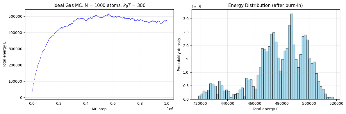
MC average energy:   <E> = 477790.9
Equipartition value: (3/2)NkT = 450000.0
Relative error: 6.18%

The Metropolis algorithm recovers the equipartition theorem!
Formalizing MCMC: Markov Chains and Detailed Balance#
The ideal gas simulation above works — but why? Why does the Metropolis algorithm produce samples from the Boltzmann distribution? The answer lies in the mathematical theory of Markov chains.
A Markov chain is a sequence of random states \(x_0, x_1, x_2, \ldots\) where the probability of the next state depends only on the current state:
The transition probability \(T(x \to x')\) defines the rules of the chain.
Stationary Distribution#
Under mild conditions (ergodicity, aperiodicity), a Markov chain converges to a unique stationary distribution \(\pi(x)\) satisfying:
This is the distribution of states after running the chain for a long time, regardless of where we started.
Detailed Balance#
A sufficient (not necessary) condition for \(\pi(x)\) to be stationary is detailed balance:
Proof that detailed balance implies stationarity:
Sum both sides over \(x\):
where we used \(\sum_x T(x' \to x) = 1\) (probability conservation). This is exactly the stationarity condition. \(\square\)
The MCMC strategy: Design \(T(x \to x')\) so that detailed balance is satisfied with \(\pi(x)\) equal to the distribution we want to sample from. The Metropolis algorithm is one such design — and the ideal gas simulation above is a specific instance of it!
The Metropolis-Hastings Algorithm#
In Lecture 12, we used the Metropolis algorithm with symmetric proposals. The Metropolis-Hastings algorithm generalizes this to asymmetric proposals.
Algorithm:
From current state \(x\), propose \(x' \sim q(x' \mid x)\) (proposal distribution)
Compute the acceptance ratio: $\(\alpha = \min\!\left(1, \; \frac{\pi(x') \, q(x \mid x')}{\pi(x) \, q(x' \mid x)}\right)\)$
Accept \(x'\) with probability \(\alpha\); otherwise stay at \(x\)
Special case — Metropolis: When \(q\) is symmetric (\(q(x' \mid x) = q(x \mid x')\)), the proposal terms cancel:
This is exactly the Metropolis algorithm from Lecture 12!
Proof: Metropolis-Hastings Satisfies Detailed Balance#
The transition probability is \(T(x \to x') = q(x' \mid x) \cdot \alpha(x \to x')\). Check detailed balance:
Case 1: \(\frac{\pi(x') q(x \mid x')}{\pi(x) q(x' \mid x)} \leq 1\), so \(\alpha(x \to x') = \frac{\pi(x') q(x \mid x')}{\pi(x) q(x' \mid x)}\) and \(\alpha(x' \to x) = 1\).
Case 2: The reverse. By symmetry of the argument, it also holds. \(\square\)
Demo: Sampling a Bimodal Distribution#
Let’s sample from a mixture of two Gaussians:
This tests the chain’s ability to jump between well-separated modes.
def target_bimodal(x):
    """Unnormalized target: mixture of two Gaussians."""
    return 0.4 * stats.norm.pdf(x, -3, 1) + 0.6 * stats.norm.pdf(x, 3, 0.5)

def metropolis_hastings(target, n_samples, x0=0.0, proposal_sigma=1.0):
    """Metropolis-Hastings with symmetric Gaussian proposal."""
    samples = np.zeros(n_samples)
    samples[0] = x0
    n_accept = 0

    for i in range(1, n_samples):
        x_current = samples[i-1]
        # Symmetric Gaussian proposal
        x_proposed = x_current + np.random.normal(0, proposal_sigma)

        # Acceptance ratio (proposal terms cancel for symmetric q)
        alpha = min(1.0, target(x_proposed) / target(x_current) )

        if np.random.uniform() < alpha:
            samples[i] = x_proposed
            n_accept += 1
        else:
            samples[i] = x_current

    return samples, n_accept / n_samples

np.random.seed(42)

# Compare three proposal widths
sigmas = [0.3, 2.0, 10.0]
results = {}

for sigma in sigmas:
    samples, acc = metropolis_hastings(target_bimodal, 50000, x0=0.0, proposal_sigma=sigma)
    results[sigma] = (samples, acc)
    print(f"sigma = {sigma:5.1f}: acceptance rate = {acc:.1%}")
sigma =   0.3: acceptance rate = 88.2%
sigma =   2.0: acceptance rate = 39.2%
sigma =  10.0: acceptance rate = 14.8%
fig, axes = plt.subplots(3, 2, figsize=(12, 9))

x_plot = np.linspace(-7, 6, 300)
p_true = target_bimodal(x_plot)

for row, sigma in enumerate(sigmas):
    samples, acc = results[sigma]

    # Left: trace plot (first 3000 steps)
    axes[row, 0].plot(samples[:3000], lw=0.5, alpha=0.7)
    axes[row, 0].set_ylabel('x')
    axes[row, 0].set_title(f'Trace: $\\sigma_q$ = {sigma}, accept = {acc:.0%}')
    axes[row, 0].grid(alpha=0.3)
    if row == 2:
        axes[row, 0].set_xlabel('Step')

    # Right: histogram vs true distribution
    axes[row, 1].hist(samples[5000:], bins=80, density=True, alpha=0.6,
                      color='skyblue', edgecolor='black')
    axes[row, 1].plot(x_plot, p_true, 'r-', lw=2, label='True $\\pi(x)$')
    axes[row, 1].set_ylabel('Density')
    axes[row, 1].set_title(f'Distribution: $\\sigma_q$ = {sigma}')
    axes[row, 1].legend(fontsize=8)
    axes[row, 1].grid(alpha=0.3)
    if row == 2:
        axes[row, 1].set_xlabel('x')

plt.tight_layout()
plt.show()

print("Observations:")
print("  σ = 0.3: High acceptance, but chain gets STUCK in one mode (poor mixing)")
print("  σ = 2.0: Moderate acceptance, good exploration of both modes (Goldilocks!)")
print("  σ = 10:  Low acceptance, chain jumps erratically (wasteful)")
print("\nRule of thumb: aim for 20-50% acceptance rate")
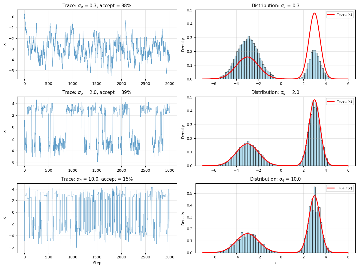
Observations:
  σ = 0.3: High acceptance, but chain gets STUCK in one mode (poor mixing)
  σ = 2.0: Moderate acceptance, good exploration of both modes (Goldilocks!)
  σ = 10:  Low acceptance, chain jumps erratically (wasteful)

Rule of thumb: aim for 20-50% acceptance rate
II. MCMC Diagnostics#
How Do We Know Our Chain Has Converged?#
MCMC produces correlated samples, unlike rejection sampling which gives i.i.d. samples. We need diagnostic tools to verify that:
The chain has reached equilibrium (burn-in is complete)
The samples are sufficiently uncorrelated for reliable estimates
The chain has explored the full distribution (mixing)
Tool 1: Burn-in#
The initial portion of the chain is influenced by the starting point and should be discarded. This is called burn-in.
Tool 2: Autocorrelation Time#
The autocorrelation function measures how correlated samples are at lag \(k\):
The integrated autocorrelation time is:
This tells us how many MCMC steps correspond to one independent sample.
Tool 3: Effective Sample Size#
From \(N\) MCMC samples, the number of effectively independent samples is:
The true standard error of the mean is:
def autocorrelation(x, max_lag=500):
    """Compute normalized autocorrelation function."""
    x = x - np.mean(x)
    n = len(x)
    var = np.var(x)
    if var == 0:
        return np.zeros(max_lag)

    acf = np.zeros(max_lag)
    for k in range(max_lag):
        acf[k] = np.mean(x[:n-k] * x[k:]) / var
    return acf

def integrated_autocorrelation_time(acf):
    """Estimate integrated autocorrelation time with automatic truncation."""
    # Truncate when ACF first goes negative (simple heuristic)
    tau = 0.5  # Start at 0.5 from the k=0 term
    for k in range(1, len(acf)):
        if acf[k] < 0:
            break
        tau += acf[k]
    return tau

def effective_sample_size(samples, max_lag=500):
    """Compute effective sample size from MCMC chain."""
    acf = autocorrelation(samples, max_lag)
    tau = integrated_autocorrelation_time(acf)
    n_eff = len(samples) / (2 * tau)
    return n_eff, tau, acf

# Analyze the three chains from above
print(f"{'σ_q':>5s}  {'N':>7s}  {'τ_int':>7s}  {'N_eff':>8s}  {'Efficiency':>11s}")
print("-" * 45)

for sigma in sigmas:
    samples = results[sigma][0][5000:]  # discard burn-in
    n_eff, tau, acf = effective_sample_size(samples)
    efficiency = n_eff / len(samples)
    print(f"{sigma:5.1f}  {len(samples):7d}  {tau:7.1f}  {n_eff:8.0f}  {efficiency:11.1%}")
  σ_q        N    τ_int     N_eff   Efficiency
---------------------------------------------
  0.3    45000    441.3        51         0.1%
  2.0    45000     42.3       532         1.2%
 10.0    45000      9.0      2492         5.5%
fig, axes = plt.subplots(1, 3, figsize=(14, 4))

colors = ['blue', 'green', 'red']

for idx, sigma in enumerate(sigmas):
    samples = results[sigma][0][5000:]
    acf = autocorrelation(samples, max_lag=200)
    axes[0].plot(acf[:200], color=colors[idx], lw=1.5, label=f'$\sigma_q$ = {sigma}')

axes[0].axhline(0, color='k', linestyle='-', alpha=0.3)
axes[0].set_xlabel('Lag k')
axes[0].set_ylabel('C(k)')
axes[0].set_title('Autocorrelation Function')
axes[0].legend(fontsize=8)
axes[0].grid(alpha=0.3)
axes[0].set_xlim(0, 200)

# Running mean convergence
for idx, sigma in enumerate(sigmas):
    samples = results[sigma][0][5000:]
    running_mean = np.cumsum(samples) / np.arange(1, len(samples)+1)
    axes[1].plot(running_mean, color=colors[idx], lw=0.8, alpha=0.8, label=f'$\sigma_q$ = {sigma}')

# True mean of bimodal distribution
x_fine = np.linspace(-8, 8, 1000)
p_fine = target_bimodal(x_fine)
true_mean = np.trapezoid(x_fine * p_fine, x_fine) / np.trapezoid(p_fine, x_fine)
axes[1].axhline(true_mean, color='k', linestyle='--', lw=2, label=f'True mean = {true_mean:.2f}')
axes[1].set_xlabel('Sample index')
axes[1].set_ylabel('Running mean')
axes[1].set_title('Running Mean Convergence')
axes[1].legend(fontsize=7)
axes[1].grid(alpha=0.3)

# Effective sample size vs proposal width
sigma_scan = np.linspace(0.1, 15, 30)
n_eff_scan = []

np.random.seed(0)
for s in sigma_scan:
    samp, _ = metropolis_hastings(target_bimodal, 10000, x0=0.0, proposal_sigma=s)
    n_eff, _, _ = effective_sample_size(samp[2000:])
    n_eff_scan.append(n_eff)

axes[2].plot(sigma_scan, n_eff_scan, 'ko-', ms=4, lw=1.5)
axes[2].set_xlabel('Proposal width $\sigma_q$')
axes[2].set_ylabel('$N_{\text{eff}}$')
axes[2].set_title('Effective Sample Size vs Proposal Width')
axes[2].grid(alpha=0.3)

idx_opt = np.argmax(n_eff_scan)
axes[2].axvline(sigma_scan[idx_opt], color='r', linestyle='--',
                label=f'Optimal $\sigma_q$ ≈ {sigma_scan[idx_opt]:.1f}')
axes[2].legend(fontsize=8)

plt.tight_layout()
plt.show()
III. Simulated Annealing#
From Sampling to Optimization#
The Metropolis algorithm samples from the Boltzmann distribution \(P(x) \propto e^{-E(x)/T}\). At low temperature, this distribution concentrates near the global minimum of \(E(x)\).
Idea: If we slowly cool the system during the Metropolis simulation, the chain will explore at high \(T\) (avoiding local minima) and then settle into the global minimum at low \(T\).
This is simulated annealing — inspired by the physical process of annealing metals.
Algorithm#
Start at high temperature \(T_0\)
Run Metropolis steps at current \(T\)
Reduce \(T\) according to a cooling schedule: \(T_{k+1} = \beta \cdot T_k\) (with \(\beta < 1\))
Repeat until \(T\) is very small
Cooling Schedule#
Common choices:
Geometric: \(T_k = T_0 \cdot \beta^k\) (most common, \(\beta \approx 0.95\)–\(0.99\))
Linear: \(T_k = T_0 - k \cdot \Delta T\)
Logarithmic: \(T_k = T_0 / \ln(1 + k)\) (provably optimal but very slow)
Theorem (Hajek, 1988): Simulated annealing converges to the global minimum with probability 1 if \(T_k \geq \frac{c}{\ln(k)}\) for sufficiently large \(c\). In practice, geometric cooling works well.
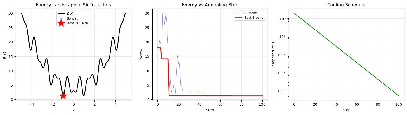
Demo: Finding the Global Minimum of a Multimodal Function#
This has many local minima. A simple gradient descent would get stuck, but simulated annealing can find the global minimum.
def energy_multimodal(x):
    """Multimodal energy landscape."""
    return x**2 + 5 * np.sin(3*x)**2 + 3 * np.cos(5*x)**2

def simulated_annealing(energy_func, x0, T0, beta, n_steps, step_size=1.0):
    """Simulated annealing with geometric cooling."""
    x = x0
    E = energy_func(x)
    x_best, E_best = x, E

    T = T0
    trajectory = [(x, E, T)]

    for step in range(n_steps):
        # Propose new state
        x_new = x + np.random.normal(0, step_size)
        E_new = energy_func(x_new)
        dE = E_new - E

        # Metropolis acceptance at temperature T
        if dE < 0 or np.random.uniform() < np.exp(-dE / T):
            x, E = x_new, E_new

            # Track best solution
            if E < E_best:
                x_best, E_best = x, E

        # Cool down
        T *= beta
        trajectory.append((x, E, T))

    return x_best, E_best, np.array(trajectory)

np.random.seed(42)

# Run SA from a bad starting point
x_best, E_best, traj = simulated_annealing(
    energy_multimodal, x0=4.0, T0=20.0, beta=0.999, n_steps=10000, step_size=1.0
)

print(f"Starting point: x = 4.0, E = {energy_multimodal(4.0):.4f}")
print(f"SA found: x = {x_best:.4f}, E = {E_best:.4f}")

# Brute force global minimum
x_grid = np.linspace(-5, 5, 10000)
E_grid = energy_multimodal(x_grid)
idx_min = np.argmin(E_grid)
print(f"Global minimum: x = {x_grid[idx_min]:.4f}, E = {E_grid[idx_min]:.4f}")
Starting point: x = 4.0, E = 17.9391
SA found: x = 0.9729, E = 1.2597
Global minimum: x = -0.9726, E = 1.2598
fig, axes = plt.subplots(1, 3, figsize=(14, 4))

# Left: energy landscape with SA trajectory
x_plot = np.linspace(-5, 5, 500)
axes[0].plot(x_plot, energy_multimodal(x_plot), 'k-', lw=2, label='$E(x)$')
axes[0].scatter(traj[::50, 0], traj[::50, 1], c=np.arange(0, len(traj), 50),
                cmap='coolwarm', s=5, alpha=0.5, label='SA path')
axes[0].plot(x_best, E_best, 'r*', ms=20, label=f'Best: x={x_best:.2f}')
axes[0].set_xlabel('x')
axes[0].set_ylabel('E(x)')
axes[0].set_title('Energy Landscape + SA Trajectory')
axes[0].legend(fontsize=8)
axes[0].grid(alpha=0.3)

# Middle: energy vs step
axes[1].plot(traj[:, 1], lw=0.5, alpha=0.7, color='blue', label='Current E')
best_so_far = np.minimum.accumulate(traj[:, 1])
axes[1].plot(best_so_far, 'r-', lw=2, label='Best E so far')
axes[1].set_xlabel('Step')
axes[1].set_ylabel('Energy')
axes[1].set_title('Energy vs Annealing Step')
axes[1].legend(fontsize=8)
axes[1].grid(alpha=0.3)

# Right: temperature schedule
axes[2].semilogy(traj[:, 2], 'g-', lw=1.5)
axes[2].set_xlabel('Step')
axes[2].set_ylabel('Temperature T')
axes[2].set_title('Cooling Schedule')
axes[2].grid(alpha=0.3)

plt.tight_layout()
plt.show()
Application: Traveling Salesman Problem (TSP)#
The Traveling Salesman Problem is a classic combinatorial optimization problem:
Given \(N\) cities with known positions, find the shortest tour that visits each city exactly once and returns to the start.
This is NP-hard — the number of possible tours is \((N-1)!/2\). For 20 cities, that’s \(\sim 10^{16}\) tours. Brute force is impossible, but simulated annealing can find near-optimal solutions.
Moves: Swap two random cities in the tour, or reverse a random segment.
import math
def tour_distance(cities, tour):
    """Total distance of a tour (closed loop)."""
    d = 0
    n = len(tour)
    for i in range(n):
        c1 = cities[tour[i]]
        c2 = cities[tour[(i+1) % n]]
        d += np.sqrt((c1[0]-c2[0])**2 + (c1[1]-c2[1])**2)
    return d

def tsp_move(tour):
    """Generate a neighboring tour by reversing a random segment."""
    new_tour = tour.copy()
    n = len(tour)
    i, j = sorted(np.random.choice(n, 2, replace=False))
    new_tour[i:j+1] = new_tour[i:j+1][::-1]  # reverse segment
    return new_tour

def tsp_annealing(cities, T0=100.0, beta=0.9995, n_steps=100000):
    """Solve TSP via simulated annealing."""
    n = len(cities)
    tour = list(range(n))
    np.random.shuffle(tour)

    E = tour_distance(cities, tour)
    best_tour, best_E = tour.copy(), E

    T = T0
    energy_history = [E]
    temp_history = [T]

    for step in range(n_steps):
        new_tour = tsp_move(tour)
        E_new = tour_distance(cities, new_tour)
        dE = E_new - E

        if dE < 0 or np.random.uniform() < np.exp(-dE / T):
            tour = new_tour
            E = E_new

            if E < best_E:
                best_tour = tour.copy()
                best_E = E

        T *= beta

        if step % 100 == 0:
            energy_history.append(E)
            temp_history.append(T)

    return best_tour, best_E, energy_history, temp_history

# Generate 25 random cities
np.random.seed(42)
n_cities = 25
cities = np.random.uniform(0, 100, size=(n_cities, 2))

# Initial random tour
initial_tour = list(range(n_cities))
initial_distance = tour_distance(cities, initial_tour)

# Solve with SA
best_tour, best_distance, energy_hist, temp_hist = tsp_annealing(
    cities, T0=100, beta=0.9995, n_steps=20000
)

print(f"Number of cities: {n_cities}")
print(f"Possible tours: {math.factorial(n_cities-1)//2:.2e}")
print(f"Initial tour distance: {initial_distance:.2f}")
print(f"SA best tour distance: {best_distance:.2f}")
print(f"Improvement: {(initial_distance - best_distance)/initial_distance:.1%}")
Number of cities: 25
Possible tours: 3.10e+23
Initial tour distance: 1373.41
SA best tour distance: 407.31
Improvement: 70.3%
def plot_tour(ax, cities, tour, title, color='blue'):
    """Plot a TSP tour."""
    tour_closed = tour + [tour[0]]  # return to start
    coords = cities[tour_closed]
    ax.plot(coords[:, 0], coords[:, 1], 'o-', color=color, ms=6, lw=1.5, alpha=0.7)
    ax.plot(cities[tour[0], 0], cities[tour[0], 1], 's', color='red', ms=10, label='Start')
    ax.set_title(title)
    ax.set_xlabel('x')
    ax.set_ylabel('y')
    ax.set_aspect('equal')
    ax.grid(alpha=0.3)

fig, axes = plt.subplots(1, 3, figsize=(15, 4))

# Left: initial tour
plot_tour(axes[0], cities, initial_tour, f'Initial Tour (d = {initial_distance:.1f})', 'gray')

# Middle: optimized tour
plot_tour(axes[1], cities, best_tour, f'SA Optimized (d = {best_distance:.1f})', 'blue')

# Right: energy convergence
axes[2].plot(energy_hist, lw=1, alpha=0.7, color='blue', label='Tour distance')
axes[2].axhline(best_distance, color='r', linestyle='--', lw=1.5, label=f'Best = {best_distance:.1f}')
axes[2].set_xlabel('Step (×100)')
axes[2].set_ylabel('Tour distance')
axes[2].set_title('SA Convergence for TSP')
axes[2].legend(fontsize=8)
axes[2].grid(alpha=0.3)

plt.tight_layout()
plt.show()

print("\nNote: SA finds a near-optimal tour in seconds, while brute force would take years!")
print("The key: high T allows uphill moves (escaping local minima), low T refines the solution.")
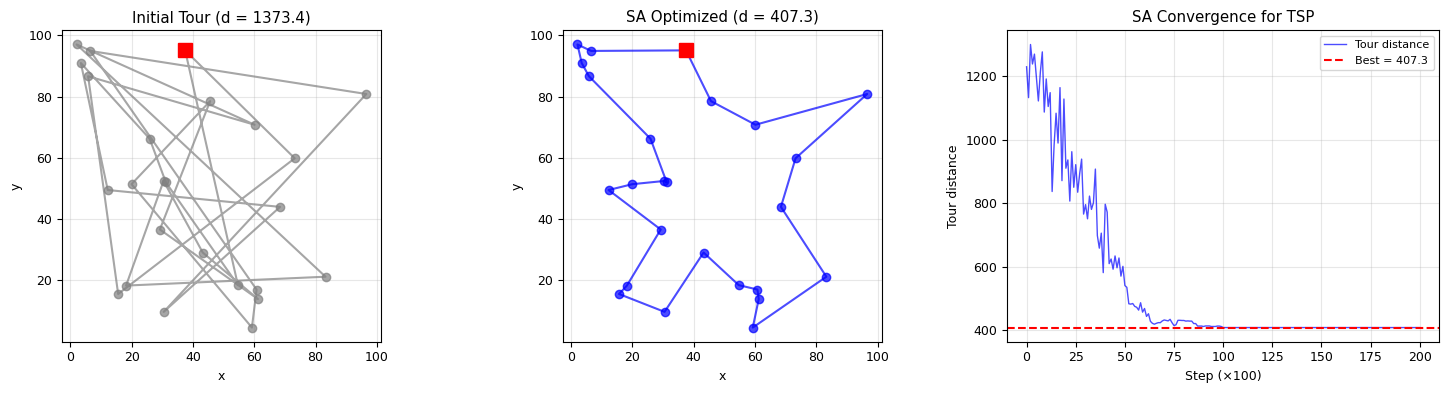
Note: SA finds a near-optimal tour in seconds, while brute force would take years!
The key: high T allows uphill moves (escaping local minima), low T refines the solution.