Lecture 22 — Machine Learning III

Deep Learning for Physics: CNNs, Autoencoders & PINNs

Computational Physics — Spring 2026

Motivation: Why Standard NNs Are Not Enough for Physics

In Lecture 21, we used MLPs — fully connected networks. They work, but:

1. Spatial structure is ignored. An MLP treats a 2D spin lattice as a flat vector — neighbouring spins have no special relationship.

2. No physics built in. The network must learn conservation laws, symmetries, and boundary conditions purely from data.

3. Data hungry. Without inductive bias, you need massive datasets.

This lecture introduces three architectures that fix these problems:

Architecture	Key idea	Physics use
CNN	Exploit spatial locality	Lattice models, field data
Autoencoder	Learn compressed representations	Order parameters, phase space
PINN	Embed PDEs in the loss	Solve ODEs/PDEs without grids

import numpy as np
import matplotlib.pyplot as plt
import torch
import torch.nn as nn
from torch.utils.data import TensorDataset, DataLoader

plt.rcParams['figure.figsize'] = [6, 4]
plt.rcParams['font.size'] = 9

device = 'cuda' if torch.cuda.is_available() else 'cpu'
print(f"PyTorch {torch.__version__}, device: {device}")

PyTorch 2.6.0, device: cpu

I. Convolutional Neural Networks (CNNs)

The Idea: Local Connectivity + Weight Sharing

Instead of connecting every input to every neuron, a CNN uses a filter (kernel) that slides across the input:

Input:   [1  0 -1  1 -1  0  1 -1]
Filter:  [1  0 -1]  (size 3)

Output:  [1*1+0*0+(-1)*(-1),  0*1+(-1)*0+1*(-1),  ...]  = [2, -1, ...]

Key properties:

1. Translation invariance: The same filter detects the same pattern anywhere

2. Local connectivity: Each output depends only on a local patch

3. Parameter efficiency: One 3x3 filter = 9 parameters, regardless of input size

For physics: lattice models, field configurations, and images all have spatial structure that CNNs can exploit.

# Visualise what a convolution does
from scipy.signal import convolve2d

# Create a simple 2D pattern (like an Ising configuration)
np.random.seed(42)
image = np.random.choice([-1, 1], size=(16, 16)).astype(float)

# Different filters detect different features
filters = {
    'Horizontal edges': np.array([[-1, -1, -1],
                                   [ 0,  0,  0],
                                   [ 1,  1,  1]]),
    'Vertical edges':   np.array([[-1, 0, 1],
                                   [-1, 0, 1],
                                   [-1, 0, 1]]),
    'Average (blur)':   np.ones((3, 3)) / 9,
    'Laplacian':        np.array([[ 0, 1, 0],
                                   [ 1,-4, 1],
                                   [ 0, 1, 0]]),
}

fig, axes = plt.subplots(1, 5, figsize=(16, 3))
axes[0].imshow(image, cmap='coolwarm')
axes[0].set_title('Input')

for ax, (name, kernel) in zip(axes[1:], filters.items()):
    result = convolve2d(image, kernel, mode='same', boundary='wrap')
    ax.imshow(result, cmap='coolwarm')
    ax.set_title(name, fontsize=8)

for ax in axes:
    ax.axis('off')

plt.suptitle('Convolution filters applied to a spin configuration', fontsize=11)
plt.tight_layout()
plt.show()

print("Note: the Laplacian filter is exactly the discrete Laplacian")
print("operator from the PDE lecture (Lecture 11)!")

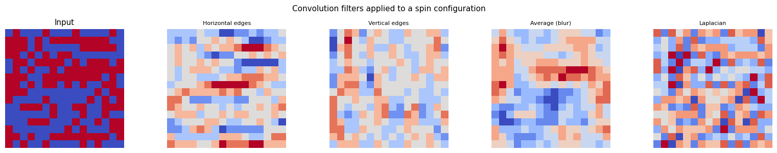
Note: the Laplacian filter is exactly the discrete Laplacian
operator from the PDE lecture (Lecture 11)!

CNN for Ising Phase Classification

In Lecture 21, we flattened the spin lattice into a vector and used logistic regression. Now we keep the 2D structure and use a CNN.

# Generate Ising data (same Metropolis sampler)
def metropolis_ising(L, T, n_sweeps=1000, n_equil=500):
    spins = np.random.choice([-1, 1], size=(L, L))
    beta = 1.0 / T
    configs = []
    for sweep in range(n_sweeps):
        for _ in range(L * L):
            i, j = np.random.randint(0, L, size=2)
            nb = (spins[(i+1)%L, j] + spins[(i-1)%L, j] +
                  spins[i, (j+1)%L] + spins[i, (j-1)%L])
            dE = 2 * spins[i, j] * nb
            if dE <= 0 or np.random.rand() < np.exp(-beta * dE):
                spins[i, j] *= -1
        if sweep >= n_equil and sweep % 10 == 0:
            configs.append(spins.copy())
    return configs

L = 16
T_c = 2.269
temps = np.concatenate([np.linspace(1.0, 2.0, 6), np.linspace(2.5, 4.0, 6)])

X_all, y_all = [], []
print("Generating Ising configurations...")
for T in temps:
    for cfg in metropolis_ising(L, T, n_sweeps=2000, n_equil=1000):
        X_all.append(cfg.astype(np.float32))
        y_all.append(0 if T < T_c else 1)

X_all = np.array(X_all)[:, np.newaxis, :, :]  # (N, 1, L, L) — channel dim
y_all = np.array(y_all)
print(f"Dataset: {X_all.shape[0]} samples, shape per sample: {X_all.shape[1:]}")

Generating Ising configurations...
Dataset: 1200 samples, shape per sample: (1, 16, 16)

from sklearn.model_selection import train_test_split

X_tr, X_te, y_tr, y_te = train_test_split(X_all, y_all, test_size=0.3, random_state=42)

X_tr_t = torch.tensor(X_tr)
y_tr_t = torch.tensor(y_tr, dtype=torch.long)
X_te_t = torch.tensor(X_te)
y_te_t = torch.tensor(y_te, dtype=torch.long)

class IsingCNN(nn.Module):
    """CNN for classifying Ising model phases."""
    def __init__(self):
        super().__init__()
        self.conv = nn.Sequential(
            # Input: (1, 16, 16)
            nn.Conv2d(1, 16, kernel_size=3, padding=1),  # (16, 16, 16)
            nn.ReLU(),
            nn.MaxPool2d(2),                              # (16, 8, 8)
            nn.Conv2d(16, 32, kernel_size=3, padding=1),  # (32, 8, 8)
            nn.ReLU(),
            nn.MaxPool2d(2),                              # (32, 4, 4)
        )
        self.fc = nn.Sequential(
            nn.Linear(32 * 4 * 4, 64),
            nn.ReLU(),
            nn.Dropout(0.3),
            nn.Linear(64, 2),
        )

    def forward(self, x):
        x = self.conv(x)
        x = x.view(x.size(0), -1)  # flatten
        return self.fc(x)

cnn = IsingCNN()
n_params_cnn = sum(p.numel() for p in cnn.parameters())
print(f"CNN parameters: {n_params_cnn}")
print(f"Compare: MLP on flattened input would need {L*L * 64} = {L*L*64} params in first layer alone")

CNN parameters: 37762
Compare: MLP on flattened input would need 16384 = 16384 params in first layer alone

# Train CNN
torch.manual_seed(42)
cnn = IsingCNN()
optimizer = torch.optim.Adam(cnn.parameters(), lr=0.001)
criterion = nn.CrossEntropyLoss()
loader = DataLoader(TensorDataset(X_tr_t, y_tr_t), batch_size=32, shuffle=True)

train_accs, test_accs = [], []
for epoch in range(30):
    cnn.train()
    for bx, by in loader:
        optimizer.zero_grad()
        criterion(cnn(bx), by).backward()
        optimizer.step()

    cnn.eval()
    with torch.no_grad():
        acc_tr = (cnn(X_tr_t).argmax(1) == y_tr_t).float().mean().item()
        acc_te = (cnn(X_te_t).argmax(1) == y_te_t).float().mean().item()
    train_accs.append(acc_tr)
    test_accs.append(acc_te)
    if epoch % 5 == 0:
        print(f"Epoch {epoch:2d}  Train: {acc_tr:.3f}  Test: {acc_te:.3f}")

print(f"\nFinal test accuracy: {test_accs[-1]:.3f}")

Epoch  0  Train: 0.993  Test: 0.992
Epoch  5  Train: 0.999  Test: 0.997
Epoch 10  Train: 1.000  Test: 0.997
Epoch 15  Train: 1.000  Test: 0.997
Epoch 20  Train: 1.000  Test: 0.997
Epoch 25  Train: 0.989  Test: 0.994

Final test accuracy: 0.997

# Visualise learned convolutional filters
filters_learned = cnn.conv[0].weight.detach().numpy()  # (16, 1, 3, 3)

fig, axes = plt.subplots(2, 8, figsize=(14, 4))
for i, ax in enumerate(axes.flat):
    ax.imshow(filters_learned[i, 0], cmap='RdBu', vmin=-0.5, vmax=0.5)
    ax.set_title(f'Filter {i}', fontsize=7)
    ax.axis('off')

plt.suptitle('First-layer CNN filters (learned from Ising data)', fontsize=11)
plt.tight_layout()
plt.show()

print("Some filters resemble edge detectors / nearest-neighbour correlators.")
print("The CNN automatically discovers physically meaningful features!")

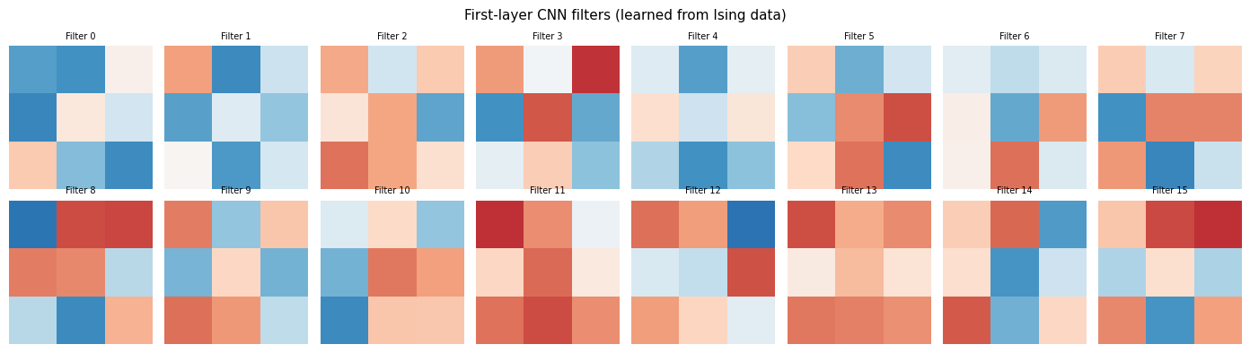
Some filters resemble edge detectors / nearest-neighbour correlators.
The CNN automatically discovers physically meaningful features!

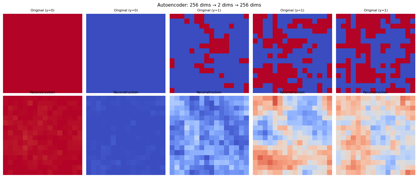
II. Autoencoders: Learning Compressed Representations

An autoencoder learns to compress data into a low-dimensional latent space and reconstruct it:

Input x  →  Encoder  →  Latent z (small!)  →  Decoder  →  Reconstructed x̂
 (256)       ↓           (2-10)                ↑           (256)
           compress                         decompress

The loss is simply \(L = \|\mathbf{x} - \hat{\mathbf{x}}\|^2\) — reconstruction error.

For physics: The latent space variables are like order parameters — the minimal set of variables needed to describe the essential physics.

class IsingAutoencoder(nn.Module):
    """Autoencoder that compresses Ising configurations to 2D latent space."""
    def __init__(self, input_dim, latent_dim=2):
        super().__init__()
        self.encoder = nn.Sequential(
            nn.Linear(input_dim, 128),
            nn.ReLU(),
            nn.Linear(128, 32),
            nn.ReLU(),
            nn.Linear(32, latent_dim),
        )
        self.decoder = nn.Sequential(
            nn.Linear(latent_dim, 32),
            nn.ReLU(),
            nn.Linear(32, 128),
            nn.ReLU(),
            nn.Linear(128, input_dim),
            nn.Tanh(),  # output in [-1, 1] like spins
        )

    def forward(self, x):
        z = self.encoder(x)
        x_hat = self.decoder(z)
        return x_hat, z

# Flatten Ising data for autoencoder
X_flat = X_all.reshape(len(X_all), -1)  # (N, 256)
X_flat_t = torch.tensor(X_flat, dtype=torch.float32)

ae = IsingAutoencoder(L * L, latent_dim=2)
print(f"Autoencoder: {L*L} → 128 → 32 → 2 → 32 → 128 → {L*L}")
print(f"Parameters: {sum(p.numel() for p in ae.parameters())}")

Autoencoder: 256 → 128 → 32 → 2 → 32 → 128 → 256
Parameters: 74434

# Train autoencoder (unsupervised — no labels!)
torch.manual_seed(42)
ae = IsingAutoencoder(L * L, latent_dim=2)
optimizer = torch.optim.Adam(ae.parameters(), lr=0.001)
loader = DataLoader(TensorDataset(X_flat_t), batch_size=64, shuffle=True)

ae_losses = []
for epoch in range(100):
    ae.train()
    epoch_loss = 0
    for (bx,) in loader:
        optimizer.zero_grad()
        x_hat, z = ae(bx)
        loss = nn.MSELoss()(x_hat, bx)
        loss.backward()
        optimizer.step()
        epoch_loss += loss.item()
    ae_losses.append(epoch_loss / len(loader))
    if epoch % 20 == 0:
        print(f"Epoch {epoch:3d}  Reconstruction loss: {ae_losses[-1]:.5f}")

Epoch   0  Reconstruction loss: 0.84789
Epoch  20  Reconstruction loss: 0.47335
Epoch  40  Reconstruction loss: 0.46386
Epoch  60  Reconstruction loss: 0.45546
Epoch  80  Reconstruction loss: 0.44664

# Show reconstructions
ae.eval()
idx = [0, len(X_all)//4, len(X_all)//2, 3*len(X_all)//4, -1]

fig, axes = plt.subplots(2, 5, figsize=(14, 6))
for i, j in enumerate(idx):
    original = X_flat[j].reshape(L, L)
    with torch.no_grad():
        recon, _ = ae(X_flat_t[[j]])  # fancy indexing — works for j=-1
    recon = recon.numpy().reshape(L, L)

    axes[0, i].imshow(original, cmap='coolwarm', vmin=-1, vmax=1)
    axes[0, i].set_title(f'Original (y={y_all[j]})', fontsize=8)
    axes[0, i].axis('off')

    axes[1, i].imshow(recon, cmap='coolwarm', vmin=-1, vmax=1)
    axes[1, i].set_title('Reconstruction', fontsize=8)
    axes[1, i].axis('off')

axes[0, 0].set_ylabel('Original', fontsize=10)
axes[1, 0].set_ylabel('Reconstructed', fontsize=10)
plt.suptitle('Autoencoder: 256 dims \u2192 2 dims \u2192 256 dims', fontsize=11)
plt.tight_layout()
plt.show()

III. Physics-Informed Neural Networks (PINNs)

The Big Idea

Instead of learning from data, we can train a neural network to satisfy a differential equation directly.

Given a PDE: $\( \mathcal{L}[u](x, t) = 0 \quad \text{(e.g., heat equation: } u_t - \alpha u_{xx} = 0\text{)} \)$

with boundary/initial conditions, we:

1. Represent the solution as a neural network: \(u(x, t) \approx u_{\theta}(x, t)\)

2. Compute derivatives \(u_t\), \(u_{xx}\) etc. using autograd (Lecture 21)

3. Minimise the physics loss:

\[ L = \underbrace{\sum_{\text{collocation}} \bigl|\mathcal{L}[u_\theta]\bigr|^2}_{\text{PDE residual}} + \lambda_{\text{BC}} \underbrace{\sum_{\text{boundary}} |u_\theta - u_{\text{BC}}|^2}_{\text{boundary conditions}} + \lambda_{\text{IC}} \underbrace{\sum_{\text{initial}} |u_\theta - u_{\text{IC}}|^2}_{\text{initial conditions}} \]

No training data needed — just the equation itself!

This connects directly to your ODE (Lecture 10) and PDE (Lecture 11) lectures, but replaces finite differences with neural networks.

Example 1: PINN Solves a Simple ODE

Let’s start simple. Solve:

\[ \frac{du}{dt} = -u, \quad u(0) = 1 \]

Exact solution: \(u(t) = e^{-t}\)

# PINN for du/dt = -u, u(0) = 1
torch.manual_seed(42)

class PINN_ODE(nn.Module):
    """PINN for solving du/dt = -u."""
    def __init__(self):
        super().__init__()
        self.net = nn.Sequential(
            nn.Linear(1, 32),
            nn.Tanh(),
            nn.Linear(32, 32),
            nn.Tanh(),
            nn.Linear(32, 1),
        )

    def forward(self, t):
        return self.net(t)

pinn_ode = PINN_ODE()
optimizer = torch.optim.Adam(pinn_ode.parameters(), lr=0.001)

# Collocation points (where we enforce the ODE)
t_col = torch.linspace(0, 5, 200, requires_grad=True).reshape(-1, 1)
# Initial condition point
t_ic = torch.tensor([[0.0]])
u_ic = torch.tensor([[1.0]])

losses_ode = []
for epoch in range(3000):
    optimizer.zero_grad()

    # PDE residual: du/dt + u = 0
    u = pinn_ode(t_col)
    du_dt = torch.autograd.grad(u.sum(), t_col, create_graph=True)[0]
    residual = du_dt + u  # should be 0
    loss_pde = (residual ** 2).mean()

    # Initial condition: u(0) = 1
    u0 = pinn_ode(t_ic)
    loss_ic = (u0 - u_ic) ** 2

    # Total loss
    loss = loss_pde + 10 * loss_ic
    loss.backward()
    optimizer.step()
    losses_ode.append(loss.item())

    if epoch % 600 == 0:
        print(f"Epoch {epoch:4d}  PDE loss: {loss_pde.item():.2e}  IC loss: {loss_ic.item():.2e}")

print(f"Final total loss: {losses_ode[-1]:.2e}")

Epoch    0  PDE loss: 7.97e-02  IC loss: 1.17e+00
Epoch  600  PDE loss: 9.08e-04  IC loss: 4.79e-08
Epoch 1200  PDE loss: 5.13e-04  IC loss: 7.37e-09
Epoch 1800  PDE loss: 2.67e-04  IC loss: 2.08e-09
Epoch 2400  PDE loss: 1.37e-04  IC loss: 5.97e-10
Final total loss: 8.15e-05

# Compare PINN solution with exact solution
t_test = torch.linspace(0, 5, 300).reshape(-1, 1)
with torch.no_grad():
    u_pinn = pinn_ode(t_test).numpy().flatten()

u_exact = np.exp(-t_test.numpy().flatten())

fig, axes = plt.subplots(1, 3, figsize=(15, 4))

axes[0].plot(t_test.numpy(), u_exact, 'k--', lw=2, label='Exact: $e^{-t}$')
axes[0].plot(t_test.numpy(), u_pinn, 'b-', lw=2, label='PINN')
axes[0].set_xlabel('t'); axes[0].set_ylabel('u(t)')
axes[0].set_title('ODE: $du/dt = -u$, $u(0)=1$')
axes[0].legend(); axes[0].grid(alpha=0.3)

axes[1].semilogy(t_test.numpy(), np.abs(u_pinn - u_exact), 'r-', lw=1.5)
axes[1].set_xlabel('t'); axes[1].set_ylabel('|Error|')
axes[1].set_title('Absolute Error')
axes[1].grid(alpha=0.3)

axes[2].semilogy(losses_ode, 'b-', alpha=0.7)
axes[2].set_xlabel('Epoch'); axes[2].set_ylabel('Loss')
axes[2].set_title('Training loss'); axes[2].grid(alpha=0.3)

plt.tight_layout()
plt.show()

print(f"Maximum error: {np.max(np.abs(u_pinn - u_exact)):.2e}")
print("The PINN learned the solution without ANY training data — just the equation!")

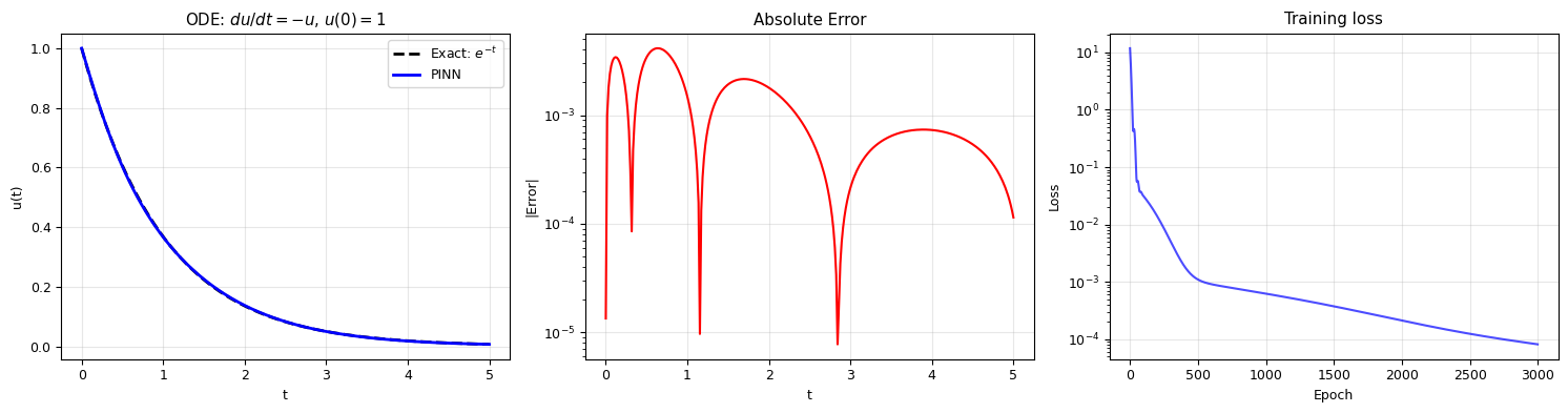
Maximum error: 4.12e-03
The PINN learned the solution without ANY training data — just the equation!

Example 2: PINN Solves a Simple Harmonic Oscillator

A more interesting ODE — the simple harmonic oscillator from Lecture 10:

\[ \frac{d^2 x}{dt^2} = -\omega^2 x, \quad x(0) = 1, \quad \dot{x}(0) = 0 \]

Exact solution: \(x(t) = \cos(\omega t)\)

This is a second-order ODE, so we need second derivatives via autograd.

# PINN for harmonic oscillator
torch.manual_seed(42)
omega = 2.0  # angular frequency

class PINN_SHO(nn.Module):
    def __init__(self):
        super().__init__()
        self.net = nn.Sequential(
            nn.Linear(1, 64),
            nn.Tanh(),
            nn.Linear(64, 64),
            nn.Tanh(),
            nn.Linear(64, 64),
            nn.Tanh(),
            nn.Linear(64, 1),
        )

    def forward(self, t):
        return self.net(t)

pinn_sho = PINN_SHO()
optimizer = torch.optim.Adam(pinn_sho.parameters(), lr=0.001)

t_col = torch.linspace(0, 4*np.pi/omega, 400).reshape(-1, 1).requires_grad_(True)

losses_sho = []
for epoch in range(5000):
    optimizer.zero_grad()

    # Forward
    x = pinn_sho(t_col)

    # First derivative dx/dt
    dx_dt = torch.autograd.grad(x.sum(), t_col, create_graph=True)[0]
    # Second derivative d²x/dt²
    d2x_dt2 = torch.autograd.grad(dx_dt.sum(), t_col, create_graph=True)[0]

    # PDE residual: d²x/dt² + ω²x = 0
    residual = d2x_dt2 + omega**2 * x
    loss_pde = (residual ** 2).mean()

    # Initial conditions: x(0)=1, dx/dt(0)=0
    t0 = torch.tensor([[0.0]], requires_grad=True)
    x0 = pinn_sho(t0)
    dx0 = torch.autograd.grad(x0, t0, create_graph=True)[0]

    loss_ic = (x0 - 1.0)**2 + dx0**2

    loss = loss_pde + 50 * loss_ic.squeeze()
    loss.backward()
    optimizer.step()
    losses_sho.append(loss.item())

    if epoch % 1000 == 0:
        print(f"Epoch {epoch:4d}  PDE: {loss_pde.item():.2e}  IC: {loss_ic.item():.2e}")

Epoch    0  PDE: 7.42e-02  IC: 1.12e+00
Epoch 1000  PDE: 3.27e-01  IC: 4.71e-05
Epoch 2000  PDE: 2.09e-01  IC: 2.33e-05
Epoch 3000  PDE: 8.85e-02  IC: 4.58e-06
Epoch 4000  PDE: 7.69e-02  IC: 2.99e-06

# Compare with exact solution
t_test = torch.linspace(0, 4*np.pi/omega, 500).reshape(-1, 1)
with torch.no_grad():
    x_pinn = pinn_sho(t_test).numpy().flatten()

x_exact = np.cos(omega * t_test.numpy().flatten())

fig, axes = plt.subplots(1, 2, figsize=(12, 4))

axes[0].plot(t_test.numpy(), x_exact, 'k--', lw=2, label=r'Exact: $\cos(\omega t)$')
axes[0].plot(t_test.numpy(), x_pinn, 'b-', lw=2, label='PINN')
axes[0].set_xlabel('t'); axes[0].set_ylabel('x(t)')
axes[0].set_title(f'Harmonic Oscillator ($\\omega$ = {omega})')
axes[0].legend(); axes[0].grid(alpha=0.3)

axes[1].semilogy(losses_sho, 'b-', alpha=0.7)
axes[1].set_xlabel('Epoch'); axes[1].set_ylabel('Loss')
axes[1].set_title('Training loss'); axes[1].grid(alpha=0.3)

plt.tight_layout()
plt.show()

print(f"Max error: {np.max(np.abs(x_pinn - x_exact)):.4f}")
print("PINN solves the harmonic oscillator with just the equation + initial conditions!")

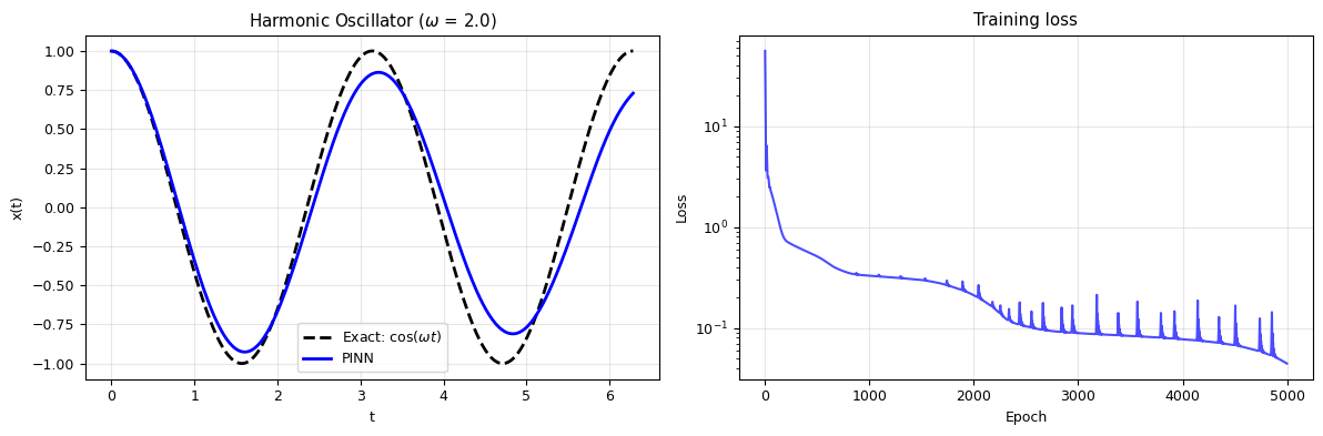
Max error: 0.3572
PINN solves the harmonic oscillator with just the equation + initial conditions!

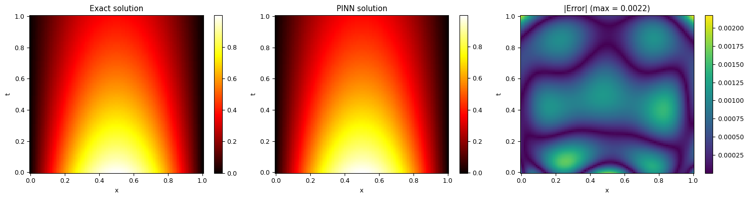
Example 3: PINN Solves the 1D Heat Equation (PDE)

Now the real power of PINNs — solving a partial differential equation.

The 1D heat equation from Lecture 11:

\[ \frac{\partial u}{\partial t} = \alpha \frac{\partial^2 u}{\partial x^2} \]

with boundary conditions \(u(0, t) = u(L, t) = 0\) and initial condition \(u(x, 0) = \sin(\pi x / L)\).

Exact solution: $\( u(x, t) = \sin\!\left(\frac{\pi x}{L}\right) \exp\!\left(-\alpha \frac{\pi^2}{L^2} t\right) \)$

Compare this with the finite-difference FTCS scheme from Lecture 11: the PINN needs no grid and handles boundaries naturally.

# PINN for the 1D heat equation
torch.manual_seed(42)

alpha_heat = 0.1  # thermal diffusivity
L_rod = 1.0       # rod length
T_final = 1.0     # simulation time

class PINN_Heat(nn.Module):
    """PINN for 1D heat equation: u_t = alpha * u_xx."""
    def __init__(self):
        super().__init__()
        self.net = nn.Sequential(
            nn.Linear(2, 64),    # input: (x, t)
            nn.Tanh(),
            nn.Linear(64, 64),
            nn.Tanh(),
            nn.Linear(64, 64),
            nn.Tanh(),
            nn.Linear(64, 1),    # output: u(x, t)
        )

    def forward(self, x, t):
        xt = torch.cat([x, t], dim=1)
        return self.net(xt)

pinn_heat = PINN_Heat()
optimizer = torch.optim.Adam(pinn_heat.parameters(), lr=0.001)

# Collocation points in the interior domain
N_col = 2000
x_col = torch.rand(N_col, 1) * L_rod
t_col = torch.rand(N_col, 1) * T_final
x_col.requires_grad_(True)
t_col.requires_grad_(True)

# Boundary condition points: u(0, t) = u(L, t) = 0
N_bc = 200
t_bc = torch.rand(N_bc, 1) * T_final
x_bc_left = torch.zeros(N_bc, 1)
x_bc_right = torch.ones(N_bc, 1) * L_rod

# Initial condition points: u(x, 0) = sin(pi*x/L)
N_ic = 200
x_ic = torch.rand(N_ic, 1) * L_rod
t_ic = torch.zeros(N_ic, 1)
u_ic = torch.sin(np.pi * x_ic / L_rod)

print(f"Collocation points: {N_col}")
print(f"Boundary points: {2 * N_bc}")
print(f"Initial condition points: {N_ic}")

Collocation points: 2000
Boundary points: 400
Initial condition points: 200

# Train the heat equation PINN
losses_heat = []

for epoch in range(5000):
    optimizer.zero_grad()

    # --- PDE residual: u_t - alpha * u_xx = 0 ---
    u = pinn_heat(x_col, t_col)

    # du/dt
    u_t = torch.autograd.grad(u.sum(), t_col, create_graph=True)[0]
    # du/dx
    u_x = torch.autograd.grad(u.sum(), x_col, create_graph=True)[0]
    # d²u/dx²
    u_xx = torch.autograd.grad(u_x.sum(), x_col, create_graph=True)[0]

    residual = u_t - alpha_heat * u_xx
    loss_pde = (residual ** 2).mean()

    # --- Boundary conditions: u(0,t) = u(L,t) = 0 ---
    u_left = pinn_heat(x_bc_left, t_bc)
    u_right = pinn_heat(x_bc_right, t_bc)
    loss_bc = (u_left ** 2).mean() + (u_right ** 2).mean()

    # --- Initial condition: u(x,0) = sin(pi*x/L) ---
    u_init = pinn_heat(x_ic, t_ic)
    loss_ic = ((u_init - u_ic) ** 2).mean()

    # Total loss
    loss = loss_pde + 10 * loss_bc + 10 * loss_ic
    loss.backward()
    optimizer.step()
    losses_heat.append(loss.item())

    if epoch % 1000 == 0:
        print(f"Epoch {epoch:4d}  PDE: {loss_pde.item():.2e}  "
              f"BC: {loss_bc.item():.2e}  IC: {loss_ic.item():.2e}")

Epoch    0  PDE: 3.34e-03  BC: 9.68e-02  IC: 7.48e-01
Epoch 1000  PDE: 3.59e-04  BC: 9.78e-05  IC: 3.99e-05
Epoch 2000  PDE: 2.10e-04  BC: 1.10e-06  IC: 7.43e-07
Epoch 3000  PDE: 1.58e-04  BC: 1.10e-06  IC: 8.01e-07
Epoch 4000  PDE: 1.38e-04  BC: 8.61e-05  IC: 3.47e-05

# Visualise PINN solution vs exact solution
def exact_heat(x, t, alpha=alpha_heat, L=L_rod):
    return np.sin(np.pi * x / L) * np.exp(-alpha * (np.pi / L)**2 * t)

# Evaluate on a grid
nx, nt = 100, 100
x_grid = np.linspace(0, L_rod, nx)
t_grid = np.linspace(0, T_final, nt)
X_grid, T_grid = np.meshgrid(x_grid, t_grid)

x_flat = torch.tensor(X_grid.flatten(), dtype=torch.float32).reshape(-1, 1)
t_flat = torch.tensor(T_grid.flatten(), dtype=torch.float32).reshape(-1, 1)

pinn_heat.eval()
with torch.no_grad():
    u_pinn = pinn_heat(x_flat, t_flat).numpy().reshape(nt, nx)

u_exact = exact_heat(X_grid, T_grid)

fig, axes = plt.subplots(1, 3, figsize=(15, 4))

im1 = axes[0].pcolormesh(X_grid, T_grid, u_exact, cmap='hot', shading='auto')
axes[0].set_xlabel('x'); axes[0].set_ylabel('t')
axes[0].set_title('Exact solution')
plt.colorbar(im1, ax=axes[0])

im2 = axes[1].pcolormesh(X_grid, T_grid, u_pinn, cmap='hot', shading='auto')
axes[1].set_xlabel('x'); axes[1].set_ylabel('t')
axes[1].set_title('PINN solution')
plt.colorbar(im2, ax=axes[1])

error = np.abs(u_pinn - u_exact)
im3 = axes[2].pcolormesh(X_grid, T_grid, error, cmap='viridis', shading='auto')
axes[2].set_xlabel('x'); axes[2].set_ylabel('t')
axes[2].set_title(f'|Error| (max = {error.max():.4f})')
plt.colorbar(im3, ax=axes[2])

plt.tight_layout()
plt.show()

# Compare PINN vs exact at specific times
fig, ax = plt.subplots(figsize=(8, 5))
times = [0, 0.1, 0.3, 0.5, 1.0]
colors = plt.cm.cool(np.linspace(0, 1, len(times)))

x_test = torch.linspace(0, L_rod, 200).reshape(-1, 1)

for t_val, color in zip(times, colors):
    t_test = torch.ones_like(x_test) * t_val
    with torch.no_grad():
        u_pinn_line = pinn_heat(x_test, t_test).numpy().flatten()
    u_exact_line = exact_heat(x_test.numpy().flatten(), t_val)

    ax.plot(x_test.numpy(), u_exact_line, '--', color=color, lw=2)
    ax.plot(x_test.numpy(), u_pinn_line, '-', color=color, lw=2,
            label=f't = {t_val}')

ax.set_xlabel('x')
ax.set_ylabel('u(x, t)')
ax.set_title('Heat Equation: PINN (solid) vs Exact (dashed)')
ax.legend()
ax.grid(alpha=0.3)
plt.tight_layout()
plt.show()

print("PINN solves the heat equation with NO grid and NO time-stepping!")
print("Compare with Lecture 11: FTCS scheme needed a grid and CFL stability condition.")

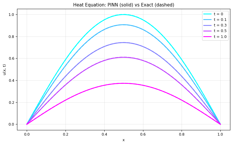
PINN solves the heat equation with NO grid and NO time-stepping!
Compare with Lecture 11: FTCS scheme needed a grid and CFL stability condition.

PINN vs Traditional Methods

Aspect	Finite Differences (Lecture 11)	PINN
Grid	Fixed grid required	Mesh-free
Stability	CFL condition constrains \(\Delta t\)	No stability issues
Dimensions	Cost grows as \(N^d\)	Cost grows slowly with \(d\)
Accuracy	Controlled by grid resolution	Controlled by network size
Irregular domains	Hard	Easy
Inverse problems	Very hard	Natural — just add unknowns

PINNs excel when: high dimensions, irregular domains, inverse problems, sparse data.
Finite differences excel when: low dimensions, high accuracy needed, simple domains.

IV. Symmetry and Equivariance

Physics is full of symmetries. If we build them into the network, it needs less data and generalises better.

Key Concepts

Invariance: Output does not change when input is transformed. $\( f(T \cdot \mathbf{x}) = f(\mathbf{x}) \)$

Example: Total energy is invariant to translation, rotation, and relabelling atoms.

Equivariance: Output transforms in the same way as the input. $\( f(T \cdot \mathbf{x}) = T \cdot f(\mathbf{x}) \)$

Example: Forces rotate with the coordinate system.

Symmetry	Invariant quantities	Equivariant quantities
Translation	Energy, pressure	Forces, momentum
Rotation	Energy, charge	Forces, angular momentum, dipole
Permutation (atom swap)	Total energy	Per-atom energies
Time reversal	Energy	Velocity

# Demo: Building permutation invariance into a network
# Problem: predict total energy from 3 pairwise distances
# The energy must not change if we swap atoms → permutation invariant

# Naive approach: just feed distances to an MLP
# Problem: MLP(r12, r13, r23) != MLP(r13, r12, r23) in general!

class NaiveMLP(nn.Module):
    def __init__(self):
        super().__init__()
        self.net = nn.Sequential(
            nn.Linear(3, 32), nn.ReLU(),
            nn.Linear(32, 1)
        )
    def forward(self, x):
        return self.net(x)

# Invariant approach: sort distances, or use symmetric aggregation
class SymmetricNN(nn.Module):
    """Process each distance independently, then sum (Deep Sets idea)."""
    def __init__(self):
        super().__init__()
        # Per-pair network
        self.phi = nn.Sequential(
            nn.Linear(1, 32), nn.ReLU(),
            nn.Linear(32, 32), nn.ReLU(),
        )
        # After summing
        self.rho = nn.Sequential(
            nn.Linear(32, 32), nn.ReLU(),
            nn.Linear(32, 1)
        )

    def forward(self, dists):
        # dists: (batch, n_pairs)
        # Process each distance independently
        per_pair = self.phi(dists.unsqueeze(-1))  # (batch, n_pairs, 32)
        # Sum over pairs (permutation invariant!)
        pooled = per_pair.sum(dim=1)  # (batch, 32)
        return self.rho(pooled)

# Test permutation invariance
torch.manual_seed(42)
naive = NaiveMLP()
symm = SymmetricNN()

test_input = torch.tensor([[1.0, 1.5, 2.0]])  # r12, r13, r23
permuted    = torch.tensor([[1.5, 1.0, 2.0]])  # r13, r12, r23 (swap atoms 2,3)

print("Naive MLP:")
print(f"  f(r12, r13, r23) = {naive(test_input).item():.4f}")
print(f"  f(r13, r12, r23) = {naive(permuted).item():.4f}")
print(f"  Different! Not invariant.\n")

print("Symmetric NN (Deep Sets):")
print(f"  f(r12, r13, r23) = {symm(test_input).item():.4f}")
print(f"  f(r13, r12, r23) = {symm(permuted).item():.4f}")
print(f"  Same! Permutation invariant by construction.")

Naive MLP:
  f(r12, r13, r23) = 0.8826
  f(r13, r12, r23) = 0.8449
  Different! Not invariant.

Symmetric NN (Deep Sets):
  f(r12, r13, r23) = 0.1557
  f(r13, r12, r23) = 0.1557
  Same! Permutation invariant by construction.

The Deep Sets Architecture

The Deep Sets theorem (Zaheer et al., 2017) states that any permutation-invariant function can be written as:

\[ f(\{x_1, \ldots, x_n\}) = \rho\!\left(\sum_{i=1}^{n} \phi(x_i)\right) \]

where \(\phi\) and \(\rho\) are learnable functions (neural networks).

This is exactly what SymmetricNN does above:

• \(\phi\): processes each element independently

• \(\sum\): symmetric aggregation

• \(\rho\): maps the aggregated representation to the output

This architecture is the foundation of Graph Neural Networks (Lecture 24).

V. Inverse Problems with PINNs

A powerful extension: what if we don’t know a parameter in the PDE?

Given noisy measurements of \(u(x, t)\), can we find the unknown diffusion coefficient \(\alpha\)?

We make \(\alpha\) a trainable parameter alongside the network weights!

# Inverse PINN: estimate diffusivity alpha from noisy observations
torch.manual_seed(42)

alpha_true = 0.1  # the value we want to recover

# Generate "experimental" observations with noise
N_obs = 100
x_obs = np.random.uniform(0.1, 0.9, N_obs)
t_obs = np.random.uniform(0.05, 0.8, N_obs)
u_obs = exact_heat(x_obs, t_obs, alpha=alpha_true) + 0.02 * np.random.randn(N_obs)

x_obs_t = torch.tensor(x_obs, dtype=torch.float32).reshape(-1, 1)
t_obs_t = torch.tensor(t_obs, dtype=torch.float32).reshape(-1, 1)
u_obs_t = torch.tensor(u_obs, dtype=torch.float32).reshape(-1, 1)

class InversePINN(nn.Module):
    def __init__(self):
        super().__init__()
        self.net = nn.Sequential(
            nn.Linear(2, 64), nn.Tanh(),
            nn.Linear(64, 64), nn.Tanh(),
            nn.Linear(64, 64), nn.Tanh(),
            nn.Linear(64, 1),
        )
        # Unknown parameter — initialise far from true value
        self.log_alpha = nn.Parameter(torch.tensor(0.0))  # alpha = exp(0) = 1.0

    @property
    def alpha(self):
        return torch.exp(self.log_alpha)  # ensure positivity

    def forward(self, x, t):
        return self.net(torch.cat([x, t], dim=1))

inv_pinn = InversePINN()
optimizer = torch.optim.Adam(inv_pinn.parameters(), lr=0.001)

# Collocation points for PDE
x_col = torch.rand(1000, 1, requires_grad=True)
t_col = torch.rand(1000, 1, requires_grad=True)

alpha_history = []
losses_inv = []

for epoch in range(5000):
    optimizer.zero_grad()

    # PDE residual
    u = inv_pinn(x_col, t_col)
    u_t = torch.autograd.grad(u.sum(), t_col, create_graph=True)[0]
    u_x = torch.autograd.grad(u.sum(), x_col, create_graph=True)[0]
    u_xx = torch.autograd.grad(u_x.sum(), x_col, create_graph=True)[0]

    residual = u_t - inv_pinn.alpha * u_xx
    loss_pde = (residual ** 2).mean()

    # Data fitting
    u_pred = inv_pinn(x_obs_t, t_obs_t)
    loss_data = ((u_pred - u_obs_t) ** 2).mean()

    # BC and IC (same as before)
    t_bc = torch.rand(100, 1)
    loss_bc = (inv_pinn(torch.zeros(100, 1), t_bc)**2).mean() + \
              (inv_pinn(torch.ones(100, 1), t_bc)**2).mean()

    x_ic = torch.rand(100, 1)
    u_ic_true = torch.sin(np.pi * x_ic)
    loss_ic = ((inv_pinn(x_ic, torch.zeros(100, 1)) - u_ic_true)**2).mean()

    loss = loss_pde + 100 * loss_data + 10 * loss_bc + 10 * loss_ic
    loss.backward()
    optimizer.step()

    alpha_history.append(inv_pinn.alpha.item())
    losses_inv.append(loss.item())

    if epoch % 1000 == 0:
        print(f"Epoch {epoch:4d}  alpha = {inv_pinn.alpha.item():.4f}  "
              f"(true: {alpha_true})  loss: {loss.item():.2e}")

print(f"\nRecovered alpha = {inv_pinn.alpha.item():.4f}")
print(f"True alpha      = {alpha_true}")
print(f"Error: {abs(inv_pinn.alpha.item() - alpha_true)/alpha_true * 100:.1f}%")

Epoch    0  alpha = 0.9990  (true: 0.1)  loss: 6.97e+01
Epoch 1000  alpha = 0.3567  (true: 0.1)  loss: 9.48e-01
Epoch 2000  alpha = 0.2086  (true: 0.1)  loss: 2.19e-01
Epoch 3000  alpha = 0.1542  (true: 0.1)  loss: 9.06e-02
Epoch 4000  alpha = 0.1266  (true: 0.1)  loss: 5.97e-02

Recovered alpha = 0.1116
True alpha      = 0.1
Error: 11.6%

fig, axes = plt.subplots(1, 2, figsize=(12, 4))

axes[0].plot(alpha_history, 'b-', lw=2)
axes[0].axhline(alpha_true, color='red', ls='--', lw=2, label=f'True $\\alpha$ = {alpha_true}')
axes[0].set_xlabel('Epoch'); axes[0].set_ylabel('$\\alpha$')
axes[0].set_title('Inverse Problem: Recovering $\\alpha$')
axes[0].legend(); axes[0].grid(alpha=0.3)

axes[1].semilogy(losses_inv, 'b-', alpha=0.5)
axes[1].set_xlabel('Epoch'); axes[1].set_ylabel('Loss')
axes[1].set_title('Training loss'); axes[1].grid(alpha=0.3)

plt.tight_layout()
plt.show()

print("The PINN recovers the unknown diffusion coefficient from noisy observations!")
print("This is extremely powerful for experimental data analysis.")

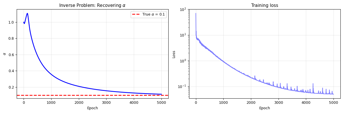
The PINN recovers the unknown diffusion coefficient from noisy observations!
This is extremely powerful for experimental data analysis.

Summary

Architecture	Key Idea	Physics Application
CNN	Exploit spatial locality via filters	Lattice models, field data
Autoencoder	Compress to low-dim latent space	Discover order parameters
PINN	Embed PDE in loss function	Solve forward and inverse problems
Deep Sets	Symmetric aggregation → invariance	Permutation-invariant energy

Next lecture: We go deeper into symmetry-aware architectures with Graph Neural Networks, where the structure of the physical system (atoms, bonds, interactions) is encoded directly in the network.