Lecture 23 — Machine Learning IV

Graph Neural Networks for Physics

Why Graphs?

Many physical systems are naturally described as graphs — a collection of nodes connected by edges:

Physical system	Nodes	Edges
Molecule	Atoms	Bonds / distance cutoff
Crystal	Atoms in unit cell	Nearest neighbours
Protein	Amino acid residues	Spatial proximity
Social network	People	Friendships
Electrical circuit	Components	Wires

The key insight: the structure of the system matters. An MLP treats inputs as a flat vector and ignores which atoms are close to which. A GNN respects the connectivity.

From Lecture 23: we built permutation-invariant networks using Deep Sets (process each element, then sum). A GNN generalises this by also considering which elements are connected.

import numpy as np
import matplotlib.pyplot as plt
import torch
import torch.nn as nn
import torch.nn.functional as F

plt.rcParams['figure.figsize'] = [6, 4]
plt.rcParams['font.size'] = 9

print(f"PyTorch {torch.__version__}")

PyTorch 2.6.0

I. Graphs: The Data Structure

A graph \(\mathbf{G} = (\mathbf{V}, \mathbf{E})\) consists of:

• Nodes \(\mathbf{V} = \{v_1, \ldots, v_N\}\) with features \(\mathbf{h}_i \in \mathbb{R}^d\)

• Edges \(\mathbf{E} = \{(i, j)\}\) with optional features \(\mathbf{e}_{ij} \in \mathbb{R}^k\)

• Neighbours of node \(i\): \(\mathbf{N}(i) = \{j : (i,j) \in \mathbf{E}\}\)

For molecular systems:

• Node features: Atomic number, element type (one-hot encoded)

• Edge features: Distance \(r_{ij}\), bond type

• Connectivity: All atom pairs within a cutoff distance \(r_c\)

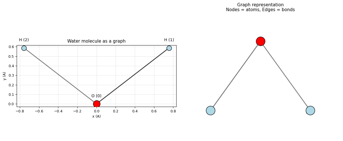
# Example: represent a water molecule as a graph
# H2O: O at center, two H atoms

# Atom positions (Angstroms)
positions = np.array([
    [0.000, 0.000, 0.000],  # O
    [0.757, 0.587, 0.000],  # H
    [-0.757, 0.587, 0.000], # H
])

atomic_numbers = [8, 1, 1]  # O, H, H
elements = ['O', 'H', 'H']

# Build graph: connect atoms within cutoff
cutoff = 2.0  # Angstroms

edges = []
edge_distances = []
for i in range(len(positions)):
    for j in range(len(positions)):
        if i != j:
            d = np.linalg.norm(positions[i] - positions[j])
            if d < cutoff:
                edges.append([i, j])
                edge_distances.append(d)

edges = np.array(edges)
edge_distances = np.array(edge_distances)

print("Water molecule graph:")
print(f"  Nodes: {len(positions)} atoms ({elements})")
print(f"  Edges: {len(edges)} connections")
for e, d in zip(edges, edge_distances):
    print(f"    {elements[e[0]]} ({e[0]}) -- {elements[e[1]]} ({e[1]}): {d:.3f} A")

Water molecule graph:
  Nodes: 3 atoms (['O', 'H', 'H'])
  Edges: 6 connections
    O (0) -- H (1): 0.958 A
    O (0) -- H (2): 0.958 A
    H (1) -- O (0): 0.958 A
    H (1) -- H (2): 1.514 A
    H (2) -- O (0): 0.958 A
    H (2) -- H (1): 1.514 A

# Visualise the molecular graph
fig, axes = plt.subplots(1, 2, figsize=(12, 5))

# 2D projection of molecule
ax = axes[0]
colors_atom = {'O': 'red', 'H': 'lightblue'}
sizes_atom = {'O': 300, 'H': 150}

for e in edges[:len(edges)//2]:  # undirected, so plot each pair once
    p1, p2 = positions[e[0]], positions[e[1]]
    ax.plot([p1[0], p2[0]], [p1[1], p2[1]], 'k-', lw=2, alpha=0.5)

for i, (pos, elem) in enumerate(zip(positions, elements)):
    ax.scatter(pos[0], pos[1], c=colors_atom[elem], s=sizes_atom[elem],
               edgecolors='black', zorder=5)
    ax.annotate(f'{elem} ({i})', (pos[0], pos[1]), fontsize=10,
                ha='center', va='bottom', xytext=(0, 15),
                textcoords='offset points')

ax.set_xlabel('x (A)'); ax.set_ylabel('y (A)')
ax.set_title('Water molecule as a graph')
ax.set_aspect('equal')
ax.grid(alpha=0.3)

# Show the graph representation schematically
ax2 = axes[1]
# Draw abstract graph
node_pos = {0: (0.5, 1), 1: (0, 0), 2: (1, 0)}
for e in edges[:len(edges)//2]:
    p1, p2 = node_pos[e[0]], node_pos[e[1]]
    ax2.annotate('', xy=p2, xytext=p1,
                 arrowprops=dict(arrowstyle='<->', color='gray', lw=2))

for i, elem in enumerate(elements):
    pos = node_pos[i]
    ax2.scatter(*pos, c=colors_atom[elem], s=500, edgecolors='black', zorder=5)
    ax2.text(pos[0], pos[1], f'{elem}\nZ={atomic_numbers[i]}',
             ha='center', va='center', fontsize=9, fontweight='bold')

ax2.set_xlim(-0.3, 1.3); ax2.set_ylim(-0.4, 1.4)
ax2.set_title('Graph representation\nNodes = atoms, Edges = bonds')
ax2.axis('off')

plt.tight_layout()
plt.show()

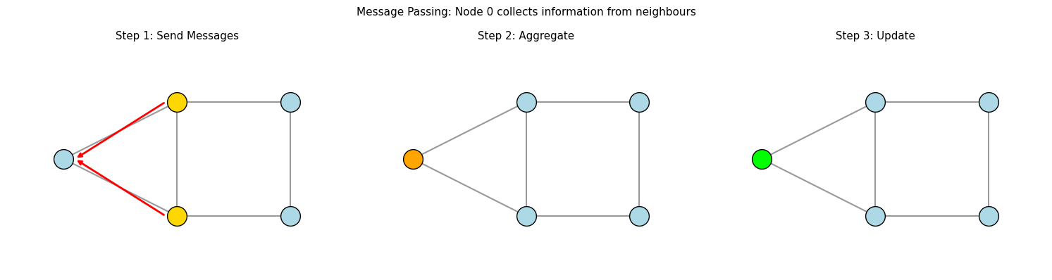
II. Message Passing: How GNNs Work

The core operation in a GNN is message passing. In each layer:

1. Message: Each node sends a message to its neighbours based on its current features

2. Aggregate: Each node collects messages from all its neighbours

3. Update: Each node updates its features based on the aggregated messages

Formally, one message-passing layer updates node \(i\)’s features as:

\[ \mathbf{h}_i^{(l+1)} = \phi\!\left( \mathbf{h}_i^{(l)},\; \bigoplus_{j \in \mathcal{N}(i)} \psi\!\left(\mathbf{h}_i^{(l)},\, \mathbf{h}_j^{(l)},\, \mathbf{e}_{ij}\right) \right) \]

where:

• \(\psi\) = message function (what information to send)

• \(\bigoplus\) = aggregation (sum, mean, or max over neighbours)

• \(\phi\) = update function (how to combine old features with messages)

After \(L\) layers, each node’s features contain information about its \(L\)-hop neighbourhood — this is the GNN’s receptive field.

# Visualise message passing
fig, axes = plt.subplots(1, 3, figsize=(15, 4))

# Simple 5-node graph
node_pos = {0: (0, 0), 1: (1, 0.5), 2: (1, -0.5), 3: (2, 0.5), 4: (2, -0.5)}
edges_vis = [(0, 1), (0, 2), (1, 3), (2, 4), (1, 2), (3, 4)]

titles = ['Step 1: Send Messages', 'Step 2: Aggregate', 'Step 3: Update']
highlights = [
    {1: 'gold', 2: 'gold'},  # messages from neighbours
    {0: 'orange'},           # aggregation at node 0
    {0: 'lime'},             # updated node
]

for ax, title, hl in zip(axes, titles, highlights):
    # Draw edges
    for (i, j) in edges_vis:
        p1, p2 = node_pos[i], node_pos[j]
        ax.plot([p1[0], p2[0]], [p1[1], p2[1]], 'k-', lw=1.5, alpha=0.4)

    # Draw nodes
    for i, pos in node_pos.items():
        color = hl.get(i, 'lightblue')
        ax.scatter(*pos, s=400, c=color, edgecolors='black', zorder=5)
        ax.text(pos[0], pos[1], str(i), ha='center', va='center', fontsize=11)

    ax.set_title(title)
    ax.set_xlim(-0.5, 2.5); ax.set_ylim(-1, 1)
    ax.axis('off')

# Add arrows for messages in step 1
for i in [1, 2]:
    p1, p2 = node_pos[i], node_pos[0]
    axes[0].annotate('', xy=(p2[0]+0.1, p2[1]), xytext=(p1[0]-0.1, p1[1]),
                     arrowprops=dict(arrowstyle='->', color='red', lw=2))

plt.suptitle('Message Passing: Node 0 collects information from neighbours', fontsize=11)
plt.tight_layout()
plt.show()

III. Building a GNN from Scratch

Let’s implement a simple message-passing GNN in pure PyTorch.

Our GNN will predict the total energy of a system of Lennard-Jones atoms from their positions and types.

class MessagePassingLayer(nn.Module):
    """
    One layer of message passing.

    For each edge (i, j):
      message_ij = MLP([h_i, h_j, e_ij])
    For each node i:
      aggregated_i = sum of messages from neighbours
      h_i_new = MLP([h_i, aggregated_i])
    """
    def __init__(self, node_dim, edge_dim, hidden_dim):
        super().__init__()
        # Message function: combines sender, receiver, and edge features
        self.message_mlp = nn.Sequential(
            nn.Linear(2 * node_dim + edge_dim, hidden_dim),
            nn.SiLU(),
            nn.Linear(hidden_dim, hidden_dim),
        )
        # Update function: combines old features with aggregated messages
        self.update_mlp = nn.Sequential(
            nn.Linear(node_dim + hidden_dim, hidden_dim),
            nn.SiLU(),
            nn.Linear(hidden_dim, node_dim),
        )

    def forward(self, h, edge_index, edge_attr):
        """
        h: (N, node_dim) node features
        edge_index: (2, E) source and target node indices
        edge_attr: (E, edge_dim) edge features
        """
        src, dst = edge_index  # source and destination nodes
        N = h.size(0)

        # 1. Compute messages
        msg_input = torch.cat([h[src], h[dst], edge_attr], dim=1)
        messages = self.message_mlp(msg_input)  # (E, hidden_dim)

        # 2. Aggregate messages (sum for each target node)
        agg = torch.zeros(N, messages.size(1), device=h.device)
        agg.index_add_(0, dst, messages)  # sum messages by target

        # 3. Update node features
        update_input = torch.cat([h, agg], dim=1)
        h_new = h + self.update_mlp(update_input)  # residual connection

        return h_new

print("MessagePassingLayer defined.")
print("Key operations: message (per edge) → aggregate (per node) → update (per node)")

MessagePassingLayer defined.
Key operations: message (per edge) → aggregate (per node) → update (per node)

class SimpleGNN(nn.Module):
    """
    Complete GNN for predicting a scalar property (like energy)
    from atomic positions.
    """
    def __init__(self, n_elements=3, node_dim=32, edge_dim=16, n_layers=3):
        super().__init__()

        # Embed atomic number into a learnable vector
        self.atom_embedding = nn.Embedding(n_elements + 1, node_dim)

        # Radial basis functions to encode distances
        self.n_rbf = edge_dim
        self.rbf_centers = nn.Parameter(
            torch.linspace(0.5, 5.0, edge_dim), requires_grad=False
        )
        self.rbf_width = 0.5

        # Message passing layers
        self.layers = nn.ModuleList([
            MessagePassingLayer(node_dim, edge_dim, node_dim)
            for _ in range(n_layers)
        ])

        # Output: per-atom energy, then sum
        self.output_mlp = nn.Sequential(
            nn.Linear(node_dim, node_dim),
            nn.SiLU(),
            nn.Linear(node_dim, 1),
        )

    def radial_basis(self, distances):
        """Expand distances into radial basis functions (Gaussian)."""
        return torch.exp(-(distances.unsqueeze(-1) - self.rbf_centers)**2
                         / (2 * self.rbf_width**2))

    def forward(self, z, positions, edge_index, batch=None):
        """
        z: (N,) atomic numbers
        positions: (N, 3) coordinates
        edge_index: (2, E) graph connectivity
        batch: (N,) which graph each atom belongs to (for batching)
        """
        # Initial node features from atom type
        h = self.atom_embedding(z)  # (N, node_dim)

        # Compute edge features from distances
        src, dst = edge_index
        diff = positions[dst] - positions[src]  # (E, 3)
        distances = torch.norm(diff, dim=1)      # (E,)
        edge_attr = self.radial_basis(distances)  # (E, n_rbf)

        # Message passing
        for layer in self.layers:
            h = layer(h, edge_index, edge_attr)

        # Per-atom energy
        atom_energy = self.output_mlp(h).squeeze(-1)  # (N,)

        # Sum per-atom energies to get total energy per molecule
        if batch is None:
            return atom_energy.sum()
        else:
            # Scatter-add by graph index
            n_graphs = batch.max().item() + 1
            energy = torch.zeros(n_graphs, device=h.device)
            energy.index_add_(0, batch, atom_energy)
            return energy

gnn = SimpleGNN()
n_params = sum(p.numel() for p in gnn.parameters())
print(f"SimpleGNN: {n_params} parameters")
print(f"Architecture: atom embedding → {len(gnn.layers)} message-passing layers → per-atom MLP → sum")

SimpleGNN: 21585 parameters
Architecture: atom embedding → 3 message-passing layers → per-atom MLP → sum

Radial Basis Functions

Distances are continuous, but neural networks work best with expanded representations. We use Gaussian radial basis functions (RBFs):

\[ \text{RBF}_k(r) = \exp\!\left(-\frac{(r - \mu_k)^2}{2\sigma^2}\right) \]

This turns a single distance into a vector of \(K\) features, each “tuned” to a different distance range.

# Visualise radial basis functions
r = torch.linspace(0, 6, 200)
centers = torch.linspace(0.5, 5.0, 16)
width = 0.5

rbf_values = torch.exp(-(r.unsqueeze(-1) - centers)**2 / (2 * width**2))

plt.figure(figsize=(8, 4))
for i in range(16):
    plt.plot(r.numpy(), rbf_values[:, i].numpy(), alpha=0.7)

plt.xlabel('Distance r (A)')
plt.ylabel('RBF value')
plt.title('Gaussian Radial Basis Functions')
plt.grid(alpha=0.3)
plt.tight_layout()
plt.show()

print(f"A distance r = 2.5 A is encoded as a {len(centers)}-dim vector:")
r_test = torch.tensor([2.5])
encoded = torch.exp(-(r_test.unsqueeze(-1) - centers)**2 / (2 * width**2))
print(f"  {encoded.numpy().round(3).flatten()}")

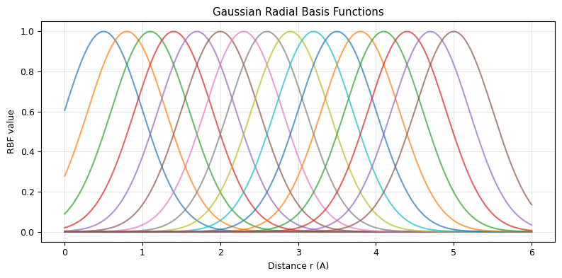
A distance r = 2.5 A is encoded as a 16-dim vector:
  [0.    0.003 0.02  0.089 0.278 0.607 0.923 0.98  0.726 0.375 0.135 0.034
 0.006 0.001 0.    0.   ]

IV. Training the GNN: Lennard-Jones Clusters

Let’s train our GNN to predict the total energy of small LJ clusters (continuing from Lecture 22).

def lj_energy(positions, epsilon=1.0, sigma=1.0):
    """Total LJ energy for a cluster."""
    N = len(positions)
    E = 0.0
    for i in range(N):
        for j in range(i+1, N):
            r = np.linalg.norm(positions[i] - positions[j])
            sr6 = (sigma / r) ** 6
            E += 4 * epsilon * (sr6**2 - sr6)
    return E

def build_graph(positions, cutoff=3.5):
    """Build edge list from positions within cutoff."""
    N = len(positions)
    src, dst = [], []
    for i in range(N):
        for j in range(N):
            if i != j:
                r = np.linalg.norm(positions[i] - positions[j])
                if r < cutoff:
                    src.append(i)
                    dst.append(j)
    return np.array([src, dst])

# Generate dataset of 4-atom LJ clusters
np.random.seed(42)
n_samples = 2000
n_atoms = 4

dataset = []
for _ in range(n_samples * 2):  # generate extra, filter bad ones
    pos = np.random.randn(n_atoms, 3) * 0.8
    # Check minimum distance
    dists = []
    for i in range(n_atoms):
        for j in range(i+1, n_atoms):
            dists.append(np.linalg.norm(pos[i] - pos[j]))
    if min(dists) < 0.8:
        continue

    E = lj_energy(pos)
    edge_index = build_graph(pos)

    dataset.append({
        'positions': pos.astype(np.float32),
        'z': np.ones(n_atoms, dtype=np.int64),  # all same atom type
        'energy': E,
        'edge_index': edge_index.astype(np.int64),
    })

    if len(dataset) >= n_samples:
        break

print(f"Generated {len(dataset)} valid clusters")
print(f"Energy range: [{min(d['energy'] for d in dataset):.2f}, {max(d['energy'] for d in dataset):.2f}]")

Generated 2000 valid clusters
Energy range: [-4.36, 77.49]

# Simple batching for GNNs
# Key trick: combine multiple graphs into one big graph with a `batch` vector

def collate_graphs(graph_list):
    """Batch multiple graphs into one big graph."""
    all_z = []
    all_pos = []
    all_edges = []
    all_energy = []
    all_batch = []

    node_offset = 0
    for i, g in enumerate(graph_list):
        N = len(g['z'])
        all_z.append(torch.tensor(g['z']))
        all_pos.append(torch.tensor(g['positions']))
        all_edges.append(torch.tensor(g['edge_index']) + node_offset)
        all_energy.append(g['energy'])
        all_batch.append(torch.full((N,), i, dtype=torch.long))
        node_offset += N

    return {
        'z': torch.cat(all_z),
        'positions': torch.cat(all_pos),
        'edge_index': torch.cat(all_edges, dim=1),
        'energy': torch.tensor(all_energy, dtype=torch.float32),
        'batch': torch.cat(all_batch),
    }

# Quick test
test_batch = collate_graphs(dataset[:3])
print("Batched graph:")
print(f"  Total nodes: {test_batch['z'].size(0)} (3 molecules x {n_atoms} atoms)")
print(f"  Total edges: {test_batch['edge_index'].size(1)}")
print(f"  Batch vector: {test_batch['batch']}")
print(f"  Energies: {test_batch['energy']}")

Batched graph:
  Total nodes: 12 (3 molecules x 4 atoms)
  Total edges: 36
  Batch vector: tensor([0, 0, 0, 0, 1, 1, 1, 1, 2, 2, 2, 2])
  Energies: tensor([56.1277, -0.7629, -1.3259])

# Train the GNN
torch.manual_seed(42)

# Split data
n_train = int(0.8 * len(dataset))
train_data = dataset[:n_train]
test_data = dataset[n_train:]

# Normalise energies
E_mean = np.mean([d['energy'] for d in train_data])
E_std = np.std([d['energy'] for d in train_data])
for d in dataset:
    d['energy_norm'] = (d['energy'] - E_mean) / E_std

# Model
gnn = SimpleGNN(n_elements=3, node_dim=32, edge_dim=16, n_layers=3)
optimizer = torch.optim.Adam(gnn.parameters(), lr=0.002)
scheduler = torch.optim.lr_scheduler.ReduceLROnPlateau(optimizer, patience=20, factor=0.5)

batch_size = 32
train_losses, val_losses = [], []

for epoch in range(200):
    gnn.train()
    np.random.shuffle(train_data)
    epoch_loss = 0
    n_batches = 0

    for i in range(0, len(train_data), batch_size):
        batch = collate_graphs(train_data[i:i+batch_size])
        optimizer.zero_grad()

        E_pred = gnn(batch['z'], batch['positions'], batch['edge_index'], batch['batch'])
        E_true = torch.tensor([d['energy_norm'] for d in train_data[i:i+batch_size]],
                              dtype=torch.float32)

        loss = F.mse_loss(E_pred, E_true)
        loss.backward()
        optimizer.step()

        epoch_loss += loss.item()
        n_batches += 1

    train_losses.append(epoch_loss / n_batches)

    # Validation
    gnn.eval()
    with torch.no_grad():
        val_batch = collate_graphs(test_data)
        E_pred_val = gnn(val_batch['z'], val_batch['positions'],
                         val_batch['edge_index'], val_batch['batch'])
        E_true_val = torch.tensor([d['energy_norm'] for d in test_data],
                                  dtype=torch.float32)
        val_loss = F.mse_loss(E_pred_val, E_true_val).item()
    val_losses.append(val_loss)
    scheduler.step(val_loss)

    if epoch % 40 == 0:
        print(f"Epoch {epoch:3d}  Train: {train_losses[-1]:.5f}  Val: {val_loss:.5f}")

print(f"\nFinal val loss: {val_losses[-1]:.5f}")

Epoch   0  Train: 1.35160  Val: 1.02464
Epoch  40  Train: 0.04884  Val: 0.03346
Epoch  80  Train: 0.03977  Val: 0.02687
Epoch 120  Train: 0.01684  Val: 0.01145
Epoch 160  Train: 0.02407  Val: 0.01994

Final val loss: 0.01001

# Evaluate: parity plot
gnn.eval()
with torch.no_grad():
    val_batch = collate_graphs(test_data)
    E_pred = gnn(val_batch['z'], val_batch['positions'],
                 val_batch['edge_index'], val_batch['batch']).numpy()

# Un-normalise
E_pred_real = E_pred * E_std + E_mean
E_true_real = np.array([d['energy'] for d in test_data])

fig, axes = plt.subplots(1, 3, figsize=(15, 4))

# Parity plot
axes[0].scatter(E_true_real, E_pred_real, s=10, alpha=0.5)
lims = [min(E_true_real.min(), E_pred_real.min()),
        max(E_true_real.max(), E_pred_real.max())]
axes[0].plot(lims, lims, 'r--', lw=2)
axes[0].set_xlabel('True Energy'); axes[0].set_ylabel('GNN Energy')
axes[0].set_title('Parity Plot'); axes[0].grid(alpha=0.3)

# Error distribution
errors = E_pred_real - E_true_real
axes[1].hist(errors, bins=40, edgecolor='black', alpha=0.7)
axes[1].set_xlabel('Error'); axes[1].set_ylabel('Count')
axes[1].set_title(f'MAE = {np.abs(errors).mean():.4f}')
axes[1].axvline(0, color='red', ls='--')

# Training curve
axes[2].semilogy(train_losses, 'b-', alpha=0.7, label='Train')
axes[2].semilogy(val_losses, 'r-', alpha=0.7, label='Val')
axes[2].set_xlabel('Epoch'); axes[2].set_ylabel('MSE')
axes[2].set_title('Training progress')
axes[2].legend(); axes[2].grid(alpha=0.3)

plt.tight_layout()
plt.show()

from sklearn.metrics import r2_score
print(f"R² = {r2_score(E_true_real, E_pred_real):.4f}")
print(f"MAE = {np.abs(errors).mean():.4f} epsilon")

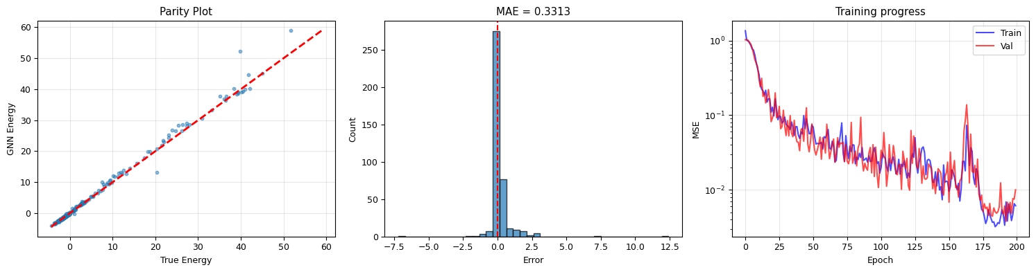
R² = 0.9902
MAE = 0.3313 epsilon

Why GNN over MLP?

Property	MLP (Lecture 22)	GNN
Input	Fixed-size vector	Variable-size graph
Permutation invariance	Must sort features	Built in (sum aggregation)
Scalability	Fixed \(N\) atoms	Any \(N\) atoms (same model!)
Locality	All-to-all	Only neighbours interact
Interpretability	Black box	Per-atom contributions

V. Equivariant GNNs: Encoding Rotational Symmetry

Our simple GNN uses distances as edge features — distances are rotation-invariant, so the predicted energy is rotation-invariant. Good!

But what about forces? Forces are vectors that rotate with the system. They are equivariant, not invariant.

The Problem

If we rotate the molecule by \(R\):

• Energy should stay the same: \(E(R\mathbf{r}) = E(\mathbf{r})\) (invariant)

• Forces should rotate: \(\mathbf{F}(R\mathbf{r}) = R\,\mathbf{F}(\mathbf{r})\) (equivariant)

Option 1: Predict energy \(E\), then compute forces via autograd: \(\mathbf{F}_i = -\nabla_{\mathbf{r}_i} E\). This is guaranteed equivariant (we used this in Lecture 22).

Option 2: Build equivariance into the network itself — this is what modern architectures like NequIP and MACE do.

# Demo: verifying rotation invariance of our GNN
torch.manual_seed(42)
gnn.eval()

# Take a test molecule
test_mol = test_data[0]
pos = torch.tensor(test_mol['positions'])
z = torch.tensor(test_mol['z'])
edge_idx = torch.tensor(test_mol['edge_index'])

# Random 3D rotation matrix
def random_rotation():
    """Generate a random 3D rotation matrix."""
    # QR decomposition of random matrix gives uniform rotation
    M = torch.randn(3, 3)
    Q, R = torch.linalg.qr(M)
    # Ensure proper rotation (det = +1)
    Q = Q * torch.sign(torch.diag(R))
    if torch.det(Q) < 0:
        Q[:, 0] *= -1
    return Q

with torch.no_grad():
    E_original = gnn(z, pos, edge_idx).item()

    print(f"Original energy: {E_original:.6f}")
    print("\nRotated energies:")
    for i in range(5):
        R = random_rotation()
        pos_rotated = pos @ R.T  # rotate all atoms
        E_rotated = gnn(z, pos_rotated, edge_idx).item()
        print(f"  Rotation {i+1}: {E_rotated:.6f}  (diff: {abs(E_rotated - E_original):.2e})")

print("\nThe GNN prediction is rotation-invariant (by construction)!")
print("This is because we only use distances, which are rotation-invariant.")

Original energy: -0.477264

Rotated energies:
  Rotation 1: -0.477264  (diff: 1.79e-07)
  Rotation 2: -0.477264  (diff: 0.00e+00)
  Rotation 3: -0.477264  (diff: 1.79e-07)
  Rotation 4: -0.477264  (diff: 1.79e-07)
  Rotation 5: -0.477264  (diff: 2.98e-07)

The GNN prediction is rotation-invariant (by construction)!
This is because we only use distances, which are rotation-invariant.

# Computing forces via autograd (equivariant by construction)
pos_grad = pos.clone().requires_grad_(True)

E = gnn(z, pos_grad, edge_idx)
E.backward()

forces = -pos_grad.grad  # F = -dE/dr

print("Forces from autograd:")
for i, (elem, f) in enumerate(zip(['A', 'A', 'A', 'A'], forces)):
    print(f"  Atom {i}: F = [{f[0]:.4f}, {f[1]:.4f}, {f[2]:.4f}]")

# Verify equivariance: rotate, then compute forces
R = random_rotation()
pos_rot = (pos @ R.T).clone().requires_grad_(True)

E_rot = gnn(z, pos_rot, edge_idx)
E_rot.backward()
forces_rot = -pos_rot.grad

# Expected: forces_rot = R @ forces
forces_expected = forces @ R.T
error = (forces_rot - forces_expected).abs().max().item()

print(f"\nForce equivariance error: {error:.2e}")
print("Forces transform correctly under rotation!")

Forces from autograd:
  Atom 0: F = [1.0334, 1.0510, 0.4401]
  Atom 1: F = [0.7535, 0.1950, 0.4841]
  Atom 2: F = [-0.6574, -0.1661, -0.6888]
  Atom 3: F = [-1.1295, -1.0799, -0.2353]

Force equivariance error: 4.95e-06
Forces transform correctly under rotation!

VI. The Landscape of Modern GNN Architectures

Our simple GNN is a good starting point, but research has produced many more powerful architectures:

Invariant Models (use distances only)

Model	Key Idea	Paper
SchNet (2017)	Continuous convolutions on distances	Schütt et al.
DimeNet (2020)	Adds angles between triplets of atoms	Gasteiger et al.
GemNet (2021)	Adds dihedral angles (4-body interactions)	Gasteiger et al.

Equivariant Models (use directional information)

Model	Key Idea	Paper
PaiNN (2021)	Equivariant message passing with vectors	Schütt et al.
NequIP (2022)	E(3)-equivariant with spherical harmonics	Batzner et al.
MACE (2022)	Multi-body equivariant messages	Batatia et al.
EquiformerV2 (2023)	Equivariant transformer	Liao et al.
EOSnet (2025)	Equivariant orbital-based many-body features (our group)	Tao and Zhu

The Key Progression

Distances only     →  + Angles          →  + Directions (vectors)
(SchNet)              (DimeNet)             (NequIP, MACE)

2-body info        →  3-body info       →  Many-body info
r_ij                  r_ij, θ_ijk           Equivariant tensor products

More geometric information → better accuracy → but more computation.

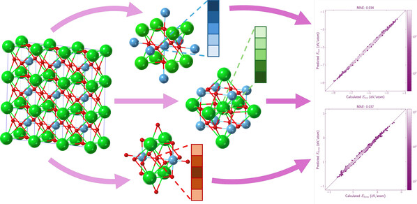
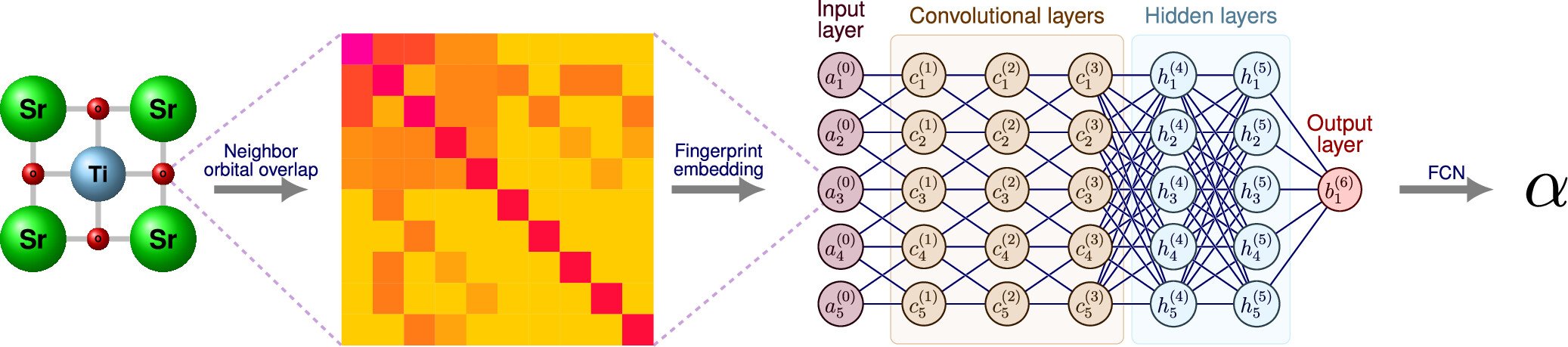
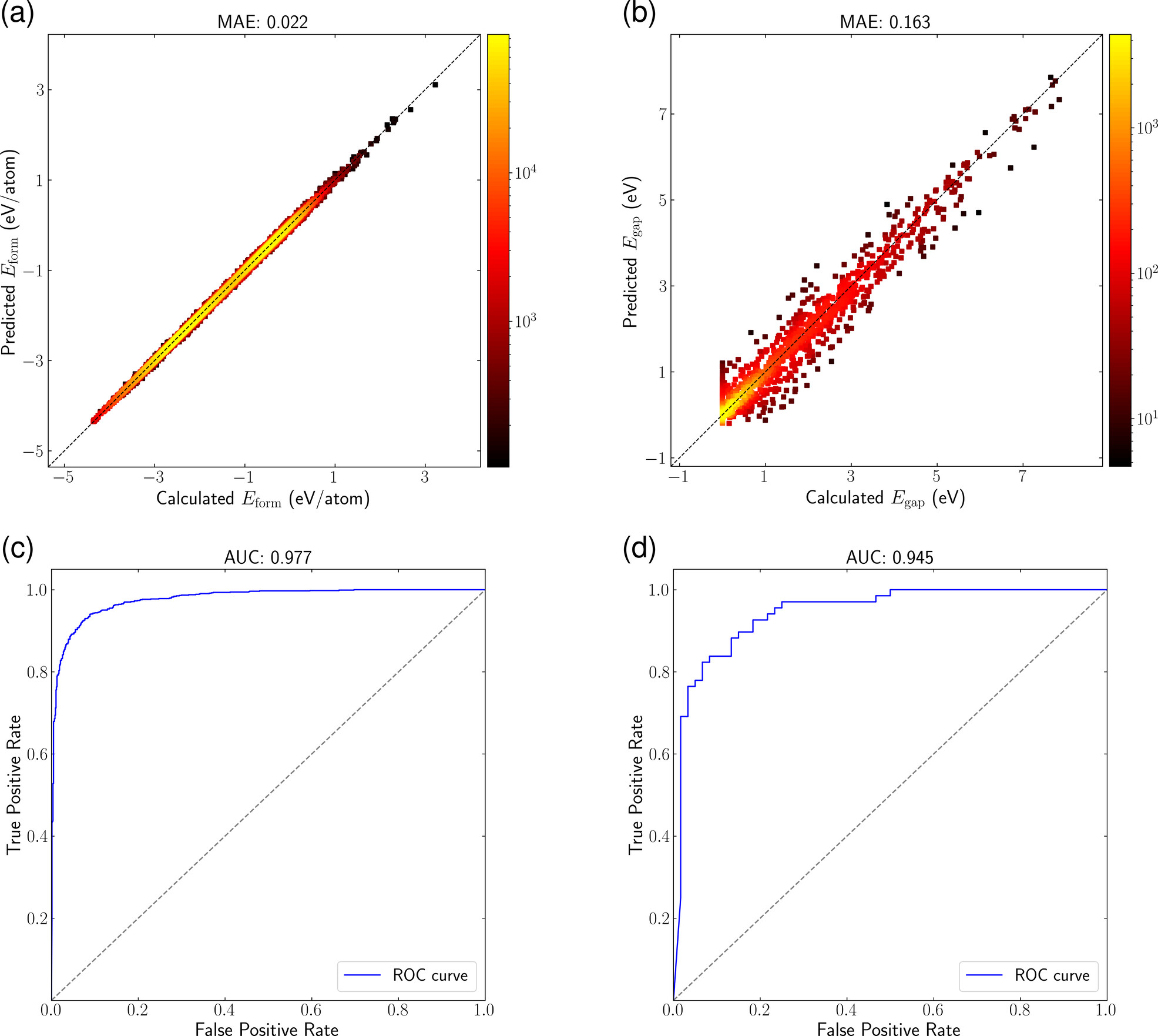
Evaluation for regression and binary classification tasks on the performance of our EOSnet model. (a) Parity plot for formation energy predictions on 131,240 data points from the Materials Project, with MAE of 0.022 eV/atom. (b) Parity plot for the prediction of electronic band gap (Eg) using 19,393 data points from the Materials Project, showing an MAE of 0.163 eV. (c) ROC curve for metal/nonmetal classification, achieving an AUC of 0.977. (d) ROC curve for dynamically stable/unstable classification on 1,335 guest-atom-substituted type-VII boron-carbide clathrates (MB6–xCx, x from 1 to 5), achieving an AUC of 0.945.

EOSnet: Rutgers-ZRG/EosNet

VII. Real-World Impact: ML Interatomic Potentials

GNN-based interatomic potentials are now a major tool in computational materials science and chemistry:

The Speed–Accuracy Trade-off

Accuracy   ↑
            |  ★ Coupled Cluster (CCSD(T))
            |  ★ DFT
            |        ★ ML Potentials (GNN)
            |                      ★ Classical Force Fields
            |-------------------------------------------→  Speed

ML potentials achieve DFT-level accuracy at force-field speed:

• DFT: ~hours for 100 atoms

• ML potential: ~milliseconds for 100 atoms

• Speedup: \(10^4\) – \(10^6\) times

Applications

Application	Method	Impact
Molecular dynamics	MACE, NequIP	Simulate millions of timesteps at DFT accuracy
Drug discovery	SchNet, DimeNet	Screen molecular properties
Materials design	MEGNet, CGCNN	Predict crystal properties
Catalysis	GemNet, EquiformerV2	Find optimal catalyst surfaces
Protein folding	GNNs in AlphaFold	Predict 3D structure from sequence

Universal ML Potentials

Recent “foundation models” for atomic systems are trained on massive DFT datasets and work across the periodic table:

• MACE-MP-0 (2023): Trained on Materials Project data, works for any element

• CHGNet (2023): Includes charge information

• M3GNet (2022): Universal potential for materials

These can be used as starting points and fine-tuned for specific systems.

VIII. Using Pre-trained GNNs with ASE

In practice, you often use pre-trained GNN potentials rather than training from scratch. The ASE (Atomic Simulation Environment) library provides a convenient interface.

Here is the typical workflow (not executed in class, but important to know):

from ase import Atoms
from ase.optimize import BFGS
## Example with MACE (if installed)
## from mace.calculators import mace_mp

## Create a molecule
water = Atoms('H2O', positions=[
    [0.0, 0.0, 0.0],
    [0.757, 0.587, 0.0],
    [-0.757, 0.587, 0.0]
])

## Attach ML calculator
## calc = mace_mp(model="medium", device="cpu")
## water.calc = calc

## Get energy and forces
## E = water.get_potential_energy()
## F = water.get_forces()

## Optimise geometry
## opt = BFGS(water)
## opt.run(fmax=0.01)

This is the same interface as DFT calculators — you can swap between ML potentials and DFT seamlessly!

IX. GNN Beyond Energy: Property Prediction

GNNs can predict many molecular/material properties beyond energy. Let’s build a simple property predictor.

# Create a synthetic dataset of "molecules" with different atom types
# and a target property that depends on composition and geometry

np.random.seed(42)

def synthetic_property(atomic_numbers, positions):
    """A synthetic property that depends on composition and geometry.
    Mimics something like a dipole moment or HOMO-LUMO gap."""
    N = len(atomic_numbers)
    # Composition term
    comp = sum(z**0.5 for z in atomic_numbers) / N
    # Geometry term (average nearest-neighbour distance)
    dists = []
    for i in range(N):
        min_d = float('inf')
        for j in range(N):
            if i != j:
                d = np.linalg.norm(positions[i] - positions[j])
                min_d = min(min_d, d)
        dists.append(min_d)
    avg_nn = np.mean(dists)
    # Property = f(composition, geometry) + noise
    return comp * avg_nn + 0.1 * np.random.randn()

# Generate molecules with 3-6 atoms, types 1-3
mol_dataset = []
for _ in range(1500):
    n_atoms = np.random.randint(3, 7)
    z = np.random.randint(1, 4, size=n_atoms)  # atom types 1, 2, 3
    pos = np.random.randn(n_atoms, 3).astype(np.float32) * 1.2

    # Check distances
    min_dist = float('inf')
    for i in range(n_atoms):
        for j in range(i+1, n_atoms):
            min_dist = min(min_dist, np.linalg.norm(pos[i] - pos[j]))
    if min_dist < 0.5:
        continue

    prop = synthetic_property(z, pos)
    edge_index = build_graph(pos, cutoff=3.5)

    mol_dataset.append({
        'z': z.astype(np.int64),
        'positions': pos,
        'edge_index': edge_index.astype(np.int64),
        'energy': prop,  # reuse 'energy' key
    })

print(f"Generated {len(mol_dataset)} molecules")
sizes = [len(d['z']) for d in mol_dataset]
print(f"Sizes: {min(sizes)}-{max(sizes)} atoms")
print(f"Property range: [{min(d['energy'] for d in mol_dataset):.2f}, "
      f"{max(d['energy'] for d in mol_dataset):.2f}]")
print("\nNote: same GNN handles molecules of DIFFERENT sizes — this is")
print("impossible with a fixed-size MLP!")

Generated 1420 molecules
Sizes: 3-6 atoms
Property range: [0.70, 7.34]

Note: same GNN handles molecules of DIFFERENT sizes — this is
impossible with a fixed-size MLP!

# Train on variable-size molecules
torch.manual_seed(42)

n_tr = int(0.8 * len(mol_dataset))
tr_mols = mol_dataset[:n_tr]
te_mols = mol_dataset[n_tr:]

# Normalise
P_mean = np.mean([d['energy'] for d in tr_mols])
P_std = np.std([d['energy'] for d in tr_mols])
for d in mol_dataset:
    d['energy_norm'] = (d['energy'] - P_mean) / P_std

gnn_prop = SimpleGNN(n_elements=4, node_dim=32, edge_dim=16, n_layers=4)
optimizer = torch.optim.Adam(gnn_prop.parameters(), lr=0.002)

batch_size = 32
train_l, val_l = [], []

for epoch in range(150):
    gnn_prop.train()
    np.random.shuffle(tr_mols)
    epoch_loss = 0
    nb = 0
    for i in range(0, len(tr_mols), batch_size):
        batch = collate_graphs(tr_mols[i:i+batch_size])
        optimizer.zero_grad()
        pred = gnn_prop(batch['z'], batch['positions'],
                        batch['edge_index'], batch['batch'])
        true = torch.tensor([d['energy_norm'] for d in tr_mols[i:i+batch_size]],
                            dtype=torch.float32)
        loss = F.mse_loss(pred, true)
        loss.backward()
        optimizer.step()
        epoch_loss += loss.item()
        nb += 1
    train_l.append(epoch_loss / nb)

    gnn_prop.eval()
    with torch.no_grad():
        vb = collate_graphs(te_mols)
        vp = gnn_prop(vb['z'], vb['positions'], vb['edge_index'], vb['batch'])
        vt = torch.tensor([d['energy_norm'] for d in te_mols], dtype=torch.float32)
        val_l.append(F.mse_loss(vp, vt).item())

    if epoch % 30 == 0:
        print(f"Epoch {epoch:3d}  Train: {train_l[-1]:.5f}  Val: {val_l[-1]:.5f}")

# Parity plot
gnn_prop.eval()
with torch.no_grad():
    vb = collate_graphs(te_mols)
    pred = gnn_prop(vb['z'], vb['positions'], vb['edge_index'], vb['batch']).numpy()

pred_real = pred * P_std + P_mean
true_real = np.array([d['energy'] for d in te_mols])

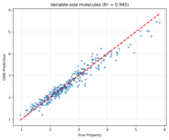
fig, ax = plt.subplots(figsize=(6, 5))
ax.scatter(true_real, pred_real, s=15, alpha=0.5)
lims = [min(true_real.min(), pred_real.min()), max(true_real.max(), pred_real.max())]
ax.plot(lims, lims, 'r--', lw=2)
ax.set_xlabel('True Property'); ax.set_ylabel('GNN Prediction')
ax.set_title(f'Variable-size molecules (R² = {r2_score(true_real, pred_real):.3f})')
ax.grid(alpha=0.3)
plt.tight_layout()
plt.show()

print("The same GNN handles 3-atom, 4-atom, 5-atom, and 6-atom molecules!")

Epoch   0  Train: 0.68437  Val: 0.52358
Epoch  30  Train: 0.07135  Val: 0.07400
Epoch  60  Train: 0.05304  Val: 0.04682
Epoch  90  Train: 0.04971  Val: 0.06432
Epoch 120  Train: 0.03480  Val: 0.07522

The same GNN handles 3-atom, 4-atom, 5-atom, and 6-atom molecules!

Summary

Concept	Key Idea
Graphs	Atoms = nodes, interactions = edges
Message passing	message → aggregate → update
Radial basis functions	Encode distances as feature vectors
Permutation invariance	Sum aggregation over neighbours
Rotation invariance	Use distances (not coordinates)
Rotation equivariance	Forces via autograd, or equivariant layers
Spherical harmonics	Basis for equivariant features
Variable size	Same model for any number of atoms

The ML for Physics Pipeline

Lecture 21: ML foundations    — Fit models, classify, evaluate
Lecture 22: Neural networks   — Learn functions, autograd for forces
Lecture 23: Physics-informed  — Embed PDEs, discover order parameters
Lecture 24: Graph networks    — Encode structure, symmetry, scalability

The big picture: ML in physics works best when we combine data with physical knowledge — symmetries, conservation laws, and the right representation of the problem.