Curve Fitting and Regression

In this lecture, we’ll learn how to find the best mathematical function to describe noisy experimental data.

Fitting vs. Interpolation

Interpolation	Curve Fitting
Passes through ALL points	Finds the best overall trend
Assumes data is exact	Accounts for noise and errors
Can oscillate wildly	Smoother, more robust
Good for tabulated data	Good for experimental data

import numpy as np
import matplotlib.pyplot as plt

# For nicer plots
plt.rcParams['figure.figsize'] = [6, 4]
plt.rcParams['font.size'] = 9

I. The Fitting Problem

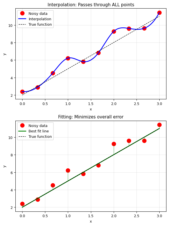
Given noisy data points \((x_1, y_1), (x_2, y_2), \ldots, (x_n, y_n)\), we want to find a function \(f(x)\) that best describes the underlying trend.

Unlike interpolation, the function does NOT need to pass through the data points. Instead, we minimize the overall error between the model and the data.

# Visualize the difference between interpolation and fitting
from scipy.interpolate import interp1d

# True underlying function
f_true = lambda x: 3*x + 2

# Generate noisy data
np.random.seed(42)
x_data = np.linspace(0, 3, 10)
y_data = f_true(x_data) + np.random.randn(10) * 0.8

# Interpolation (passes through all points)
f_interp = interp1d(x_data, y_data, kind='cubic')
x_fine = np.linspace(0, 3, 200)

plt.figure(figsize=(6, 8))

plt.subplot(2, 1, 1)
plt.plot(x_data, y_data, 'ro', markersize=10, label='Noisy data')
plt.plot(x_fine, f_interp(x_fine), 'b-', linewidth=2, label='Interpolation')
plt.plot(x_fine, f_true(x_fine), 'k--', linewidth=1, label='True function')
plt.xlabel('x')
plt.ylabel('y')
plt.title('Interpolation: Passes through ALL points')
plt.legend()
plt.grid(True, alpha=0.3)

plt.subplot(2, 1, 2)
plt.plot(x_data, y_data, 'ro', markersize=10, label='Noisy data')
plt.plot(x_fine, f_true(x_fine), 'g-', linewidth=2, label='Best fit line')
plt.plot(x_fine, f_true(x_fine), 'k--', linewidth=1, label='True function')
# Show residuals
for i in range(len(x_data)):
    plt.plot([x_data[i], x_data[i]], [y_data[i], f_true(x_data[i])],
             'g-', alpha=0.5, linewidth=1)
plt.xlabel('x')
plt.ylabel('y')
plt.title('Fitting: Minimizes overall error')
plt.legend()
plt.grid(True, alpha=0.3)

plt.tight_layout()
plt.show()

print('Interpolation follows every bump in the noise.')
print('Fitting captures the TRUE underlying trend.')

Interpolation follows every bump in the noise.
Fitting captures the TRUE underlying trend.

II. The Least Squares Principle

What is the “best” fit?

We need a criterion. The most common is least squares: minimize the sum of squared residuals.

Given data \((x_i, y_i)\) and a model \(f(x)\), the error (or cost function) is:

\[\text{err} = \sum_{i=1}^{n} \left( y_i - f(x_i) \right)^2\]

The best fit is the one that minimizes this error.

Why squared differences?

• Positive and negative errors don’t cancel out

• Larger errors are penalized more heavily

• The math works out nicely (differentiable, has unique minimum)

• Related to maximum likelihood estimation for Gaussian noise

III. Linear Fitting (from Scratch)

The Simplest Case: \(f(x) = ax + b\)

We want to find the slope \(a\) and intercept \(b\) that minimize:

\[\text{err}(a, b) = \sum_{i=1}^{n} \left( y_i - (a x_i + b) \right)^2\]

Deriving the Solution

At the minimum, the partial derivatives must be zero:

\[\frac{\partial \text{err}}{\partial a} = -2\sum_{i=1}^{n} x_i \left( y_i - a x_i - b \right) = 0\]

\[\frac{\partial \text{err}}{\partial b} = -2\sum_{i=1}^{n} \left( y_i - a x_i - b \right) = 0\]

These give us a system of two linear equations:

\[a \sum x_i^2 + b \sum x_i = \sum x_i y_i\]

\[a \sum x_i + b \cdot n = \sum y_i\]

Matrix Form

This can be written as \(\mathbf{A} \vec{p} = \vec{c}\):

\[\begin{split}\begin{bmatrix} n & \sum x_i \\ \sum x_i & \sum x_i^2 \end{bmatrix} \begin{bmatrix} b \\ a \end{bmatrix} = \begin{bmatrix} \sum y_i \\ \sum x_i y_i \end{bmatrix}\end{split}\]

This is just solving \(\mathbf{A}\vec{p} = \vec{c}\)!

# Implement linear fitting from scratch
def linear_fit(x, y):
    """
    Linear least squares fit: y = a*x + b
    Implemented from scratch using the normal equations.

    Parameters:
        x, y: arrays of data points

    Returns:
        a (slope), b (intercept)
    """
    n = len(x)

    # Compute the sums we need
    sum_x = np.sum(x)
    sum_y = np.sum(y)
    sum_x2 = np.sum(x**2)
    sum_xy = np.sum(x*y)

    # Build the matrix equation: A @ [b, a] = c
    A = np.array([ [n, sum_x],
                  [sum_x, sum_x2]
    ])

    c = np.array([sum_y, sum_xy])

    # Solve A @ p = c
    p = np.linalg.solve(A, c)

    b, a = p  # p = [b, a]
    return a, b

# Test with our noisy data
a_fit, b_fit = linear_fit(x_data, y_data)

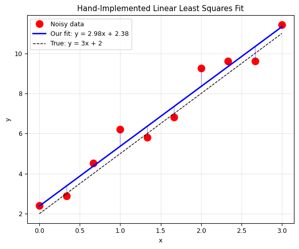
print(f'True parameters:   a = 3.000, b = 2.000')
print(f'Fitted parameters: a = {a_fit:.3f}, b = {b_fit:.3f}')

# Plot
plt.figure(figsize=(6, 5))
plt.plot(x_data, y_data, 'ro', markersize=10, label='Noisy data')
plt.plot(x_fine, a_fit * x_fine + b_fit, 'b-', linewidth=2,
         label=f'Our fit: y = {a_fit:.2f}x + {b_fit:.2f}')
plt.plot(x_fine, f_true(x_fine), 'k--', linewidth=1, label='True: y = 3x + 2')

# Show residuals
for i in range(len(x_data)):
    y_pred = a_fit * x_data[i] + b_fit
    plt.plot([x_data[i], x_data[i]], [y_data[i], y_pred],
             'b-', alpha=0.4, linewidth=1)

plt.xlabel('x')
plt.ylabel('y')
plt.title('Hand-Implemented Linear Least Squares Fit')
plt.legend()
plt.grid(True, alpha=0.3)
plt.tight_layout()
plt.show()

True parameters:   a = 3.000, b = 2.000
Fitted parameters: a = 2.983, b = 2.383

Alternative: Using scipy.optimize.minimize

We can also find the fit by directly minimizing the error function numerically:

# Method 2: Using scipy.optimize.minimize
from scipy.optimize import minimize

# Define the model function
def fit_func(x, a, b):
    return a * x + b

# Define the error (cost) function
def err_func(params, x, y):
    """Sum of squared residuals."""
    a, b = params
    y_pred = fit_func(x, a, b)
    err = np.sum((y - y_pred)**2)
    return err

# Minimize!
param_init = [1.0, 1.0]  # Initial guess
result = minimize(err_func, param_init, args=(x_data, y_data))

a_opt, b_opt = result.x
print(f'Our analytic solution:  a = {a_fit:.4f}, b = {b_fit:.4f}')
print(f'scipy.optimize result:  a = {a_opt:.4f}, b = {b_opt:.4f}')
print(f'\nThey match! Both methods give the same answer.')
print(f'\nMinimum error: {result.fun:.4f}')
print(f'Optimization converged: {result.success}')

Our analytic solution:  a = 2.9834, b = 2.3833
scipy.optimize result:  a = 2.9834, b = 2.3833

They match! Both methods give the same answer.

Minimum error: 3.0085
Optimization converged: True

IV. Polynomial Fitting

Generalizing to Higher-Order Polynomials

For a polynomial of degree \(j\): \(f(x) = a_0 + a_1 x + a_2 x^2 + \cdots + a_j x^j\)

The least squares condition leads to the normal equations in matrix form:

\[\begin{split}\begin{pmatrix} n & \sum x_i & \sum x_i^2 & \cdots & \sum x_i^j \\ \sum x_i & \sum x_i^2 & \sum x_i^3 & \cdots & \sum x_i^{j+1} \\ \sum x_i^2 & \sum x_i^3 & \sum x_i^4 & \cdots & \sum x_i^{j+2} \\ \vdots & & & \ddots & \vdots \\ \sum x_i^j & \sum x_i^{j+1} & \sum x_i^{j+2} & \cdots & \sum x_i^{2j} \end{pmatrix} \begin{pmatrix} a_0 \\ a_1 \\ a_2 \\ \vdots \\ a_j \end{pmatrix} = \begin{pmatrix} \sum y_i \\ \sum x_i y_i \\ \sum x_i^2 y_i \\ \vdots \\ \sum x_i^j y_i \end{pmatrix}\end{split}\]

This is again \(\mathbf{A}\vec{p} = \vec{c}\), where \(\mathbf{A}\) is a (j+1) × (j+1) matrix.

Note

The matrix \(\mathbf{A}\) is called the Vandermonde matrix and can become ill-conditioned for high polynomial degrees.

# Implement polynomial fitting from scratch
def poly_fit_manual(x, y, degree):
    """
    Polynomial least squares fit - implemented from scratch.

    Parameters:
        x, y: arrays of data points
        degree: degree of the polynomial

    Returns:
        coefficients [a0, a1, a2, ...]
    """
    n = degree + 1  # Number of coefficients

    # Build the normal equation matrix A
    A = np.zeros((n, n))
    for row in range(n):
        for col in range(n):
            # code..
            # A[row, col] = ...
            A[row, col] = np.sum(x**(row+col))

    # Build the right-hand side vector c
    c = np.zeros(n)
    for row in range(n):
        # code ..
        # c[row] = ...
        c[row] = np.sum(y*x**row)


    # Solve for coefficients
    coeffs = np.linalg.solve(A, c)
    return coeffs  # [a0, a1, a2, ...]

def poly_eval(coeffs, x):
    """Evaluate polynomial given coefficients [a0, a1, a2, ...]."""
    result = np.zeros_like(x, dtype=float)
    for i, a in enumerate(coeffs):
        result += a * x**i
    return result

# Generate quadratic data with noise
np.random.seed(42)
x_poly = np.linspace(0, 10, 50)
y_poly = 2*x_poly**2 + 3*x_poly + 4 + np.random.normal(0, 10, 50)

# Fit with our hand-implemented function
coeffs = poly_fit_manual(x_poly, y_poly, 2)
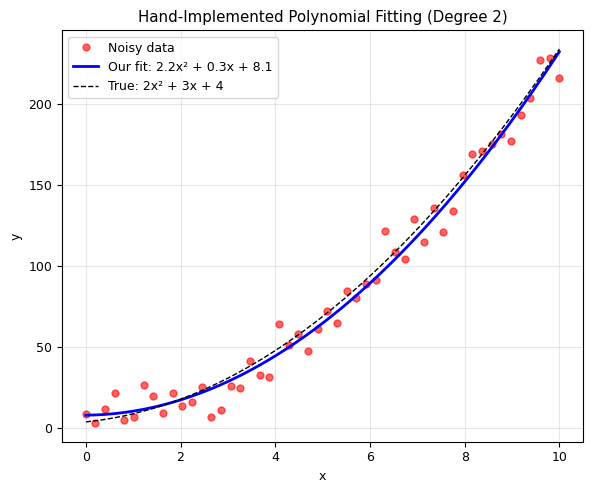
print(f'True coefficients:   a0 = 4, a1 = 3, a2 = 2')
print(f'Fitted coefficients: a0 = {coeffs[0]:.2f}, a1 = {coeffs[1]:.2f}, a2 = {coeffs[2]:.2f}')

# Plot
x_plot = np.linspace(0, 10, 200)
plt.figure(figsize=(6, 5))
plt.plot(x_poly, y_poly, 'ro', markersize=5, alpha=0.6, label='Noisy data')
plt.plot(x_plot, poly_eval(coeffs, x_plot), 'b-', linewidth=2,
         label=f'Our fit: {coeffs[2]:.1f}x² + {coeffs[1]:.1f}x + {coeffs[0]:.1f}')
plt.plot(x_plot, 2*x_plot**2 + 3*x_plot + 4, 'k--', linewidth=1,
         label='True: 2x² + 3x + 4')
plt.xlabel('x')
plt.ylabel('y')
plt.title('Hand-Implemented Polynomial Fitting (Degree 2)')
plt.legend()
plt.grid(True, alpha=0.3)
plt.tight_layout()
plt.show()

True coefficients:   a0 = 4, a1 = 3, a2 = 2
Fitted coefficients: a0 = 8.14, a1 = 0.28, a2 = 2.21

Using np.polyfit from NumPy

NumPy provides np.polyfit(x, y, degree) for polynomial fitting, and np.polyval(p, x) for evaluation.

# Compare our result with numpy's polyfit
p_numpy = np.polyfit(x_poly, y_poly, 2)  # Returns [a2, a1, a0] (highest first!)

print('Our implementation: a0={:.2f}, a1={:.2f}, a2={:.2f}'.format(*coeffs))
print('np.polyfit:         a0={:.2f}, a1={:.2f}, a2={:.2f}'.format(p_numpy[2], p_numpy[1], p_numpy[0]))
print('\nNote: np.polyfit returns coefficients in REVERSE order (highest degree first)!')

Our implementation: a0=8.14, a1=0.28, a2=2.21
np.polyfit:         a0=8.14, a1=0.28, a2=2.21

Note: np.polyfit returns coefficients in REVERSE order (highest degree first)!

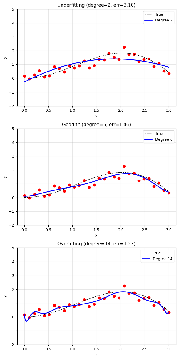
Choosing the Right Polynomial Degree

Quiz: Try different polynomial degrees. Which one gives the best fit?

# Effect of polynomial degree: underfitting vs overfitting
f_complex = lambda x: x * np.sin(x)

np.random.seed(42)
x_demo = np.linspace(0, 3, 30)
y_demo = f_complex(x_demo) + 0.3 * np.random.randn(30)
x_fine_demo = np.linspace(0, 3, 200)

plt.figure(figsize=(6, 12))

for idx, order in enumerate([2, 6, 14]):
    plt.subplot(3, 1, idx + 1)

    fit = np.polyfit(x_demo, y_demo, order)
    y_pred = np.polyval(fit, x_fine_demo)

    # Compute residual
    y_pred_data = np.polyval(fit, x_demo)
    residual = np.sum((y_demo - y_pred_data)**2)

    plt.plot(x_demo, y_demo, 'ro', markersize=6)
    plt.plot(x_fine_demo, f_complex(x_fine_demo), 'k--', linewidth=1, label='True')
    plt.plot(x_fine_demo, y_pred, 'b-', linewidth=2, label=f'Degree {order}')
    plt.xlabel('x')
    plt.ylabel('y')

    title = ['Underfitting', 'Good fit', 'Overfitting'][idx]
    plt.title(f'{title} (degree={order}, err={residual:.2f})')
    plt.legend()
    plt.grid(True, alpha=0.3)
    plt.ylim(-2, 5)

plt.tight_layout()
plt.show()

print('Underfitting: Model too simple — misses the trend')
print('Overfitting:  Model too complex — fits the noise, not the signal')
print('Good fit:     Right balance — captures the trend, ignores the noise')

Underfitting: Model too simple — misses the trend
Overfitting:  Model too complex — fits the noise, not the signal
Good fit:     Right balance — captures the trend, ignores the noise

V. General Curve Fitting

What if the model is not a polynomial? For example:

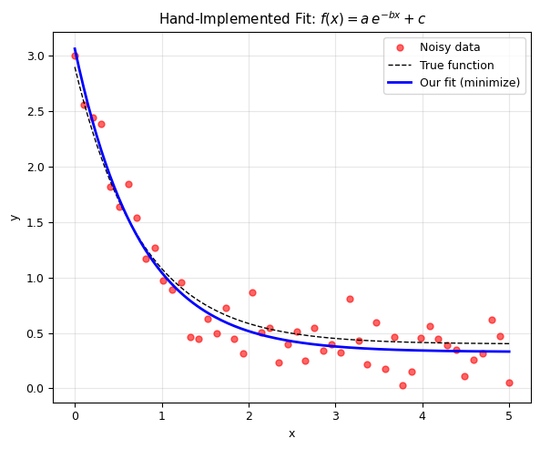
• Exponential decay: \(f(x) = a \, e^{-bx} + c\)

• Gaussian: \(f(x) = \frac{1}{\sqrt{2\pi\sigma^2}} e^{-(x-\mu)^2/(2\sigma^2)}\)

• Power law: \(f(x) = a \, x^b\)

• Sinusoidal: \(f(x) = A \sin(\omega x + \phi)\)

Two Approaches

1. scipy.optimize.minimize — Define an error function and minimize it (we already know this!)

2. scipy.optimize.curve_fit — A convenient wrapper designed specifically for fitting

Method 1: Using scipy.optimize.minimize (by hand)

# Example: Fit an exponential decay f(x) = a * exp(-b*x) + c
from scipy.optimize import minimize

# Generate data
np.random.seed(42)
a_true, b_true, c_true = 2.5, 1.3, 0.4
x_exp = np.linspace(0, 5, 50)
y_exp = a_true * np.exp(-b_true * x_exp) + c_true + 0.2 * np.random.randn(50)

# Step 1: Define the model function
def exp_model(x, a, b, c):
    return a * np.exp(-b * x) + c

# Step 2: Define the error function
def err_exp(params, x, y):
    a, b, c = params
    y_pred = exp_model(x, a, b, c)
    return np.sum((y - y_pred)**2)

# Step 3: Minimize!
param_init = [1.0, 1.0, 0.0]  # Initial guess
result = minimize(err_exp, param_init, args=(x_exp, y_exp))
a_fit, b_fit, c_fit = result.x

print('True parameters:    a={:.3f}, b={:.3f}, c={:.3f}'.format(a_true, b_true, c_true))
print('Fitted parameters:  a={:.3f}, b={:.3f}, c={:.3f}'.format(a_fit, b_fit, c_fit))

# Plot
x_plot = np.linspace(0, 5, 200)
plt.figure(figsize=(6, 5))
plt.plot(x_exp, y_exp, 'ro', markersize=5, alpha=0.6, label='Noisy data')
plt.plot(x_plot, exp_model(x_plot, a_true, b_true, c_true), 'k--', linewidth=1, label='True function')
plt.plot(x_plot, exp_model(x_plot, a_fit, b_fit, c_fit), 'b-', linewidth=2, label='Our fit (minimize)')
plt.xlabel('x')
plt.ylabel('y')
plt.title(r'Hand-Implemented Fit: $f(x) = a \, e^{-bx} + c$')
plt.legend()
plt.grid(True, alpha=0.3)
plt.tight_layout()
plt.show()

True parameters:    a=2.500, b=1.300, c=0.400
Fitted parameters:  a=2.736, b=1.339, c=0.329

Method 2: Using scipy.optimize.curve_fit

curve_fit is a convenient function designed specifically for fitting. It:

• Takes the model function, x data, and y data

• Returns optimal parameters AND their covariance matrix (uncertainty!)

from scipy.optimize import curve_fit

# curve_fit expects f(x, param1, param2, ...)
# It returns (optimal_params, covariance_matrix)
params_cf, covariance = curve_fit(exp_model, x_exp, y_exp, p0=[1, 1, 0])

# Extract parameter uncertainties from covariance matrix
uncertainties = np.sqrt(np.diag(covariance))

print('curve_fit results:')
print(f'  a = {params_cf[0]:.4f} +/- {uncertainties[0]:.4f}')
print(f'  b = {params_cf[1]:.4f} +/- {uncertainties[1]:.4f}')
print(f'  c = {params_cf[2]:.4f} +/- {uncertainties[2]:.4f}')
print(f'\nTrue values: a={a_true}, b={b_true}, c={c_true}')
print('\nAdvantage of curve_fit: it gives you uncertainties automatically!')

curve_fit results:
  a = 2.7355 +/- 0.1188
  b = 1.3390 +/- 0.1132
  c = 0.3289 +/- 0.0396

True values: a=2.5, b=1.3, c=0.4

Advantage of curve_fit: it gives you uncertainties automatically!

Example: Gaussian Fitting

Fitting a Gaussian peak is very common in spectroscopy, particle physics, and signal processing.

# Gaussian fitting example
def gaussian(x, A, mu, sigma):
    """Gaussian function with amplitude A, center mu, width sigma."""
    return A * np.exp(-(x - mu)**2 / (2 * sigma**2))

# Generate data
np.random.seed(42)
x_gauss = np.linspace(-10, 10, 100)
y_gauss = gaussian(x_gauss, 5.0, 1.5, 2.0) + 0.2 * np.random.randn(100)

# Fit
params_gauss, cov_gauss = curve_fit(gaussian, x_gauss, y_gauss, p0=[4, 0, 1])
A_fit, mu_fit, sigma_fit = params_gauss
errs = np.sqrt(np.diag(cov_gauss))

# Plot
plt.figure(figsize=(6, 5))
plt.plot(x_gauss, y_gauss, 'ko', markersize=4, alpha=0.5, label='Data')
plt.plot(x_gauss, gaussian(x_gauss, *params_gauss), 'r-', linewidth=2,
         label=f'Fit: A={A_fit:.2f}, $\\mu$={mu_fit:.2f}, $\\sigma$={sigma_fit:.2f}')
plt.axvline(mu_fit, color='g', linestyle='--', alpha=0.5, label=f'Center: $\\mu$ = {mu_fit:.2f}')
plt.xlabel('x')
plt.ylabel('y')
plt.title('Gaussian Curve Fitting')
plt.legend()
plt.grid(True, alpha=0.3)
plt.tight_layout()
plt.show()

print(f'Fitted: A = {A_fit:.3f} +/- {errs[0]:.3f}')
print(f'        mu = {mu_fit:.3f} +/- {errs[1]:.3f}')
print(f'        sigma = {sigma_fit:.3f} +/- {errs[2]:.3f}')
print(f'True:   A = 5.000, mu = 1.500, sigma = 2.000')

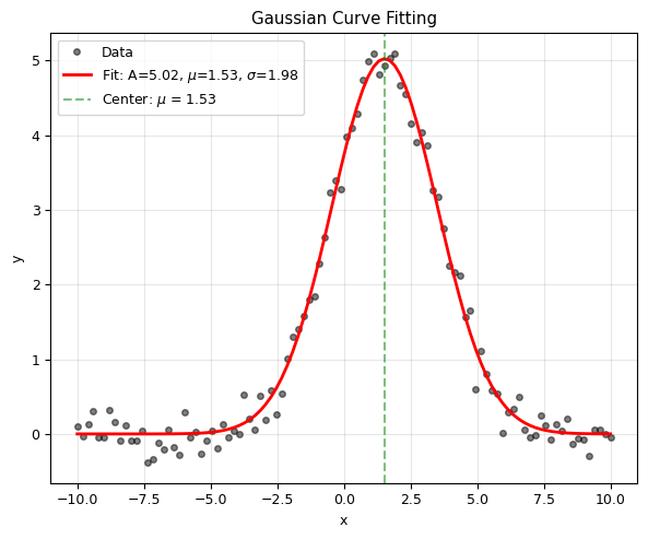
Fitted: A = 5.024 +/- 0.054
        mu = 1.531 +/- 0.024
        sigma = 1.980 +/- 0.024
True:   A = 5.000, mu = 1.500, sigma = 2.000

VI. Goodness of Fit

How do we know if our fit is good? Several metrics:

Residual Sum of Squares (RSS)

\[\text{RSS} = \sum_{i=1}^{n} (y_i - f(x_i))^2\]

Coefficient of Determination (\(R^2\))

\[R^2 = 1 - \frac{\text{RSS}}{\text{TSS}} = 1 - \frac{\sum(y_i - f(x_i))^2}{\sum(y_i - \bar{y})^2}\]

where TSS = Total Sum of Squares.

• \(R^2 = 1\): Perfect fit

• \(R^2 = 0\): Model no better than the mean

• \(R^2 < 0\): Model is worse than the mean!

Reduced Chi-Squared (\(\chi^2_\nu\))

\[\chi^2_\nu = \frac{1}{n - p} \sum_{i=1}^{n} \frac{(y_i - f(x_i))^2}{\sigma_i^2}\]

where \(p\) = number of parameters, \(\sigma_i\) = measurement uncertainty.

• \(\chi^2_\nu \approx 1\): Good fit

• \(\chi^2_\nu \gg 1\): Poor fit (or underestimated uncertainties)

• \(\chi^2_\nu \ll 1\): Overfitting (or overestimated uncertainties)

def compute_r_squared(y_data, y_pred):
    """Compute R² (coefficient of determination)."""
    ss_res = np.sum((y_data - y_pred)**2)  # Residual sum of squares
    ss_tot = np.sum((y_data - np.mean(y_data))**2)  # Total sum of squares
    return 1 - ss_res / ss_tot

# Compare R² for different polynomial degrees
print('R² for different polynomial degrees:')
print('=' * 40)
for degree in range(1, 8):
    p = np.polyfit(x_demo, y_demo, degree)
    y_pred = np.polyval(p, x_demo)
    r2 = compute_r_squared(y_demo, y_pred)
    print(f'  Degree {degree}: R² = {r2:.6f}')

print('\nNote: R² always increases with degree (more parameters)!')
print('But higher R² does NOT always mean a better model.')
print('Use adjusted R² or cross-validation to avoid overfitting.')

R² for different polynomial degrees:
========================================
  Degree 1: R² = 0.315799
  Degree 2: R² = 0.679083
  Degree 3: R² = 0.827932
  Degree 4: R² = 0.834795
  Degree 5: R² = 0.841264
  Degree 6: R² = 0.848789
  Degree 7: R² = 0.852316

Note: R² always increases with degree (more parameters)!
But higher R² does NOT always mean a better model.
Use adjusted R² or cross-validation to avoid overfitting.

Residual Analysis

A good fit should have random residuals. Patterns in residuals indicate a poor model.

# Residual analysis: linear vs quadratic fit on quadratic data
np.random.seed(42)
x_res = np.linspace(0, 5, 30)
y_res = 0.5 * x_res**2 - x_res + 1 + 0.5 * np.random.randn(30)

# Linear fit
p_lin = np.polyfit(x_res, y_res, 1)
residuals_lin = y_res - np.polyval(p_lin, x_res)

# Quadratic fit
p_quad = np.polyfit(x_res, y_res, 2)
residuals_quad = y_res - np.polyval(p_quad, x_res)

fig, axes = plt.subplots(2, 2, figsize=(6, 8))

# Linear fit
axes[0, 0].plot(x_res, y_res, 'ro', markersize=5)
axes[0, 0].plot(x_res, np.polyval(p_lin, x_res), 'b-', linewidth=2)
axes[0, 0].set_title(f'Linear Fit (R² = {compute_r_squared(y_res, np.polyval(p_lin, x_res)):.4f})', fontsize=9)
axes[0, 0].set_xlabel('x')
axes[0, 0].set_ylabel('y')
axes[0, 0].grid(True, alpha=0.3)

axes[0, 1].stem(x_res, residuals_lin, linefmt='b-', markerfmt='bo', basefmt='k-')
axes[0, 1].axhline(0, color='r', linestyle='--')
axes[0, 1].set_title('Residuals: Clear pattern!', fontsize=9)
axes[0, 1].set_xlabel('x')
axes[0, 1].set_ylabel('Residual')
axes[0, 1].grid(True, alpha=0.3)

# Quadratic fit
axes[1, 0].plot(x_res, y_res, 'ro', markersize=5)
axes[1, 0].plot(x_res, np.polyval(p_quad, x_res), 'g-', linewidth=2)
axes[1, 0].set_title(f'Quadratic Fit (R² = {compute_r_squared(y_res, np.polyval(p_quad, x_res)):.4f})', fontsize=9)
axes[1, 0].set_xlabel('x')
axes[1, 0].set_ylabel('y')
axes[1, 0].grid(True, alpha=0.3)

axes[1, 1].stem(x_res, residuals_quad, linefmt='g-', markerfmt='go', basefmt='k-')
axes[1, 1].axhline(0, color='r', linestyle='--')
axes[1, 1].set_title('Residuals: Random scatter!', fontsize=9)
axes[1, 1].set_xlabel('x')
axes[1, 1].set_ylabel('Residual')
axes[1, 1].grid(True, alpha=0.3)

plt.tight_layout()
plt.show()

print('Linear fit: Residuals show a pattern -> wrong model!')
print('Quadratic fit: Residuals are random -> good model!')

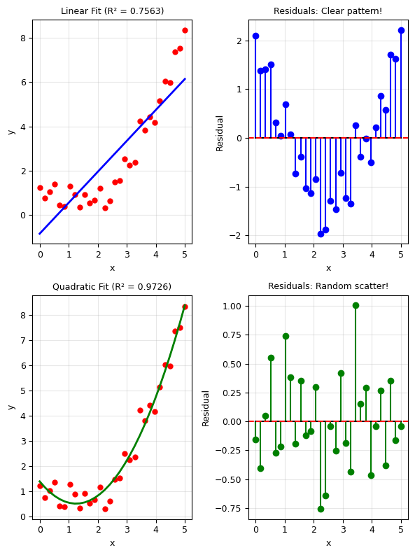
Linear fit: Residuals show a pattern -> wrong model!
Quadratic fit: Residuals are random -> good model!

VII. Distance Metrics: Beyond Least Squares

The least squares (\(L_2\) norm) is the most common, but not the only option:

\(L_p\) Distances

\[\text{err}_{L_p} = \left( \sum_{i=1}^{n} |y_i - f(x_i)|^p \right)^{1/p}\]

Distance Metrics

Distance	Properties
\(L_1\) (Manhattan)	Robust to outliers
\(L_2\) (Euclidean)	Most common, smooth
\(L_\infty\) (Chebyshev)	Minimizes worst case

\(L_1\) (Manhattan)

\[ \sum_i |y_i - f(x_i)| \]

\(L_2\) (Euclidean)
$\( \sqrt{\sum_i (y_i - f(x_i))^2} \)$

\(L_\infty\) (Chebyshev)

\[ \max_i |y_i - f(x_i)| \]

When to use which?

• \(L_2\): Default choice, best for Gaussian noise

• \(L_1\): When data has outliers (more robust)

• \(L_\infty\): When worst-case error matters

# Demonstrate L1 vs L2 with outliers
np.random.seed(42)
x_out = np.linspace(0, 5, 20)
y_out = 2 * x_out + 1 + 0.5 * np.random.randn(20)

# Add outliers
y_out[5] = 20   # Far from trend
y_out[15] = -5   # Far from trend

# L2 fit (standard least squares)
p_L2 = np.polyfit(x_out, y_out, 1)

# L1 fit (minimize absolute deviations)
def err_L1(params, x, y):
    a, b = params
    return np.sum(np.abs(y - (a * x + b)))

result_L1 = minimize(err_L1, [1, 1], args=(x_out, y_out), method='Nelder-Mead')
a_L1, b_L1 = result_L1.x

plt.figure(figsize=(6, 5))
plt.plot(x_out, y_out, 'ko', markersize=8, label='Data (with outliers)')
plt.plot(x_out[5], y_out[5], 'rx', markersize=12, markeredgewidth=3)
plt.plot(x_out[15], y_out[15], 'rx', markersize=12, markeredgewidth=3)
plt.plot(x_out, np.polyval(p_L2, x_out), 'b-', linewidth=2,
         label=f'L2 fit: y = {p_L2[0]:.2f}x + {p_L2[1]:.2f}')
plt.plot(x_out, a_L1 * x_out + b_L1, 'r--', linewidth=2,
         label=f'L1 fit: y = {a_L1:.2f}x + {b_L1:.2f}')
plt.plot(x_out, 2 * x_out + 1, 'g:', linewidth=2, label='True: y = 2x + 1')

plt.xlabel('x')
plt.ylabel('y')
plt.title('L1 vs L2 Fitting with Outliers')
plt.legend()
plt.grid(True, alpha=0.3)
plt.tight_layout()
plt.show()

print('L2 is pulled toward the outliers (sensitive to large errors).')
print('L1 is more robust — closer to the true line despite outliers.')

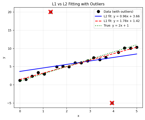
L2 is pulled toward the outliers (sensitive to large errors).
L1 is more robust — closer to the true line despite outliers.

VIII. Physics Applications

1. Radioactive Decay

Radioactive decay follows: \(N(t) = N_0 \, e^{-\lambda t}\)

where \(\lambda\) is the decay constant and \(t_{1/2} = \ln 2 / \lambda\).

# Radioactive decay fitting
def decay_model(t, N0, lam):
    return N0 * np.exp(-lam * t)

# Simulate "experimental" data
np.random.seed(42)
N0_true, lam_true = 1000, 0.1  # True parameters
t_data = np.linspace(0, 30, 15)
N_data = decay_model(t_data, N0_true, lam_true) + 20 * np.random.randn(15)
N_data = np.maximum(N_data, 0)  # Can't have negative counts

# Fit
params_decay, cov_decay = curve_fit(decay_model, t_data, N_data, p0=[800, 0.05])
N0_fit, lam_fit = params_decay
errs_decay = np.sqrt(np.diag(cov_decay))

# Calculate half-life
half_life = np.log(2) / lam_fit
half_life_err = np.log(2) / lam_fit**2 * errs_decay[1]  # Error propagation

# Plot
t_fine = np.linspace(0, 30, 200)
plt.figure(figsize=(6, 5))
plt.plot(t_data, N_data, 'ro', markersize=8, label='Measured counts')
plt.plot(t_fine, decay_model(t_fine, *params_decay), 'b-', linewidth=2,
         label=f'Fit: $N_0$={N0_fit:.0f}, $\\lambda$={lam_fit:.4f}')
plt.axvline(half_life, color='g', linestyle='--', alpha=0.7,
            label=f'Half-life = {half_life:.1f} ± {half_life_err:.1f} s')
plt.xlabel('Time (s)')
plt.ylabel('Counts')
plt.title('Radioactive Decay Fitting')
plt.legend()
plt.grid(True, alpha=0.3)
plt.tight_layout()
plt.show()

print(f'True:   N0 = {N0_true}, lambda = {lam_true}, half-life = {np.log(2)/lam_true:.2f} s')
print(f'Fitted: N0 = {N0_fit:.1f} +/- {errs_decay[0]:.1f}')
print(f'        lambda = {lam_fit:.4f} +/- {errs_decay[1]:.4f}')
print(f'        half-life = {half_life:.2f} +/- {half_life_err:.2f} s')

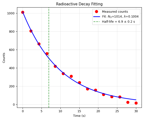
True:   N0 = 1000, lambda = 0.1, half-life = 6.93 s
Fitted: N0 = 1013.6 +/- 15.2
        lambda = 0.1004 +/- 0.0024
        half-life = 6.91 +/- 0.17 s

2. Damped Oscillation

A damped oscillator: \(x(t) = A \, e^{-\gamma t} \cos(\omega t + \phi)\)

# Damped oscillation fitting
def damped_oscillation(t, A, gamma, omega, phi):
    return A * np.exp(-gamma * t) * np.cos(omega * t + phi)

# Simulate data
np.random.seed(42)
A_true, gamma_true, omega_true, phi_true = 5.0, 0.3, 4.0, 0.5
t_osc = np.linspace(0, 10, 80)
x_osc = damped_oscillation(t_osc, A_true, gamma_true, omega_true, phi_true)
x_osc_noisy = x_osc + 0.3 * np.random.randn(len(t_osc))

# Fit
params_osc, cov_osc = curve_fit(damped_oscillation, t_osc, x_osc_noisy,
                                 p0=[4, 0.2, 3.5, 0])
A_fit, gamma_fit, omega_fit, phi_fit = params_osc

# Plot
t_fine = np.linspace(0, 10, 500)
plt.figure(figsize=(6, 5))
plt.plot(t_osc, x_osc_noisy, 'ko', markersize=4, alpha=0.5, label='Noisy data')
plt.plot(t_fine, damped_oscillation(t_fine, *params_osc), 'r-', linewidth=2, label='Fit')
plt.plot(t_fine, A_fit * np.exp(-gamma_fit * t_fine), 'b--', linewidth=1,
         alpha=0.7, label='Envelope')
plt.plot(t_fine, -A_fit * np.exp(-gamma_fit * t_fine), 'b--', linewidth=1, alpha=0.7)
plt.xlabel('Time (s)')
plt.ylabel('Displacement (m)')
plt.title(r'Damped Oscillation: $x(t) = A e^{-\gamma t} \cos(\omega t + \phi)$')
plt.legend()
plt.grid(True, alpha=0.3)
plt.tight_layout()
plt.show()

print(f'Fitted parameters:')
print(f'  Amplitude A = {A_fit:.3f} (true: {A_true})')
print(f'  Damping gamma = {gamma_fit:.3f} s^-1 (true: {gamma_true})')
print(f'  Frequency omega = {omega_fit:.3f} rad/s (true: {omega_true})')
print(f'  Phase phi = {phi_fit:.3f} rad (true: {phi_true})')
print(f'\n  Quality factor Q = omega/(2*gamma) = {omega_fit/(2*gamma_fit):.2f}')

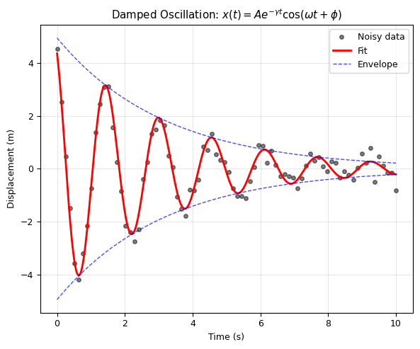
Fitted parameters:
  Amplitude A = 4.941 (true: 5.0)
  Damping gamma = 0.314 s^-1 (true: 0.3)
  Frequency omega = 4.014 rad/s (true: 4.0)
  Phase phi = 0.493 rad (true: 0.5)

  Quality factor Q = omega/(2*gamma) = 6.40

3. Power Law: Kepler’s Third Law

Kepler’s Third Law: \(T^2 = a^3\) (in appropriate units)

Or equivalently: \(T = C \cdot a^{3/2}\), which is a power law!

# Kepler's Third Law
def power_law(x, C, n):
    return C * x**n

# Planetary data
planet_names = ['Mercury', 'Venus', 'Earth', 'Mars', 'Jupiter', 'Saturn']
a_AU = np.array([0.39, 0.72, 1.00, 1.52, 5.20, 9.54])  # Semi-major axis (AU)
T_yr = np.array([0.24, 0.62, 1.00, 1.88, 11.86, 29.46])  # Period (years)

# Fit power law T = C * a^n
params_kepler, cov_kepler = curve_fit(power_law, a_AU, T_yr, p0=[1, 1.5])
C_fit, n_fit = params_kepler
errs_kepler = np.sqrt(np.diag(cov_kepler))

fig, axes = plt.subplots(2, 1, figsize=(6, 8))

# Linear plot
a_fine = np.linspace(0.1, 10, 100)
axes[0].plot(a_AU, T_yr, 'ro', markersize=10)
for i, name in enumerate(planet_names):
    axes[0].annotate(name, (a_AU[i], T_yr[i]), textcoords='offset points',
                     xytext=(10, 5), fontsize=9)
axes[0].plot(a_fine, power_law(a_fine, *params_kepler), 'b-', linewidth=2,
             label=f'Fit: T = {C_fit:.3f} a^{{{n_fit:.3f}}}')
axes[0].set_xlabel('Semi-major axis (AU)')
axes[0].set_ylabel('Orbital period (years)')
axes[0].set_title("Kepler's Third Law")
axes[0].legend()
axes[0].grid(True, alpha=0.3)

# Log-log plot (power law becomes a straight line!)
axes[1].loglog(a_AU, T_yr, 'ro', markersize=10)
axes[1].loglog(a_fine, power_law(a_fine, *params_kepler), 'b-', linewidth=2,
               label=f'Slope = {n_fit:.3f} (expected: 1.500)')
axes[1].set_xlabel('Semi-major axis (AU)')
axes[1].set_ylabel('Orbital period (years)')
axes[1].set_title('Log-Log Plot: Power Law = Straight Line')
axes[1].legend()
axes[1].grid(True, alpha=0.3)

plt.tight_layout()
plt.show()

print(f"Fitted: T = {C_fit:.4f} * a^{n_fit:.4f}")
print(f"Expected (Kepler): T = 1.000 * a^1.500")
print(f"\nFitted exponent: {n_fit:.4f} +/- {errs_kepler[1]:.4f}")
print(f"Deviation from 3/2: {abs(n_fit - 1.5):.4f}")
print(f"\nKepler's Third Law confirmed!")

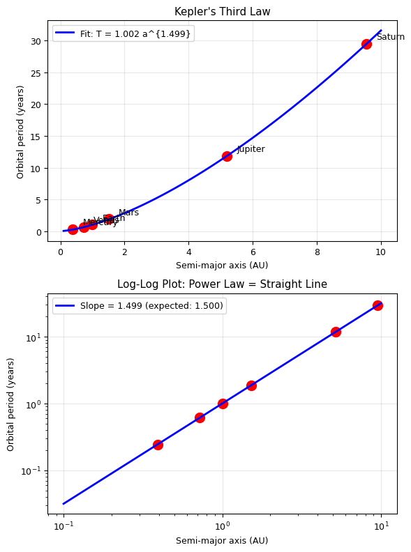
Fitted: T = 1.0020 * a^1.4990
Expected (Kepler): T = 1.000 * a^1.500

Fitted exponent: 1.4990 +/- 0.0006
Deviation from 3/2: 0.0010

Kepler's Third Law confirmed!

4. Econophysics: Bitcoin Power Law

Econophysics applies methods from statistical physics to financial systems. It’s a recognized branch of physics studied at institutions worldwide since the 1990s.

Power laws appear throughout econophysics:

• Wealth distribution (Pareto’s Law)

• Price return distributions (fat tails)

• Network growth effects (Metcalfe’s Law)

A remarkable empirical observation: Bitcoin’s price appears to follow a power law in time:

\[P(t) = a \cdot t^n\]

where \(t\) is time (days since Bitcoin’s creation). On a log-log plot, this should appear as a straight line.

Key question: Is this a fundamental “law” like Kepler’s, or just an empirical trend?

# Econophysics: Bitcoin Power Law Fitting
# Historical Bitcoin price data (monthly averages, selected points)
# Source: publicly available Bitcoin price history

# Days since Bitcoin genesis block (Jan 3, 2009)
# Selected data points spanning 2010-2024
btc_days = np.array([
    365,    # Jan 2010
    545,    # Jul 2010
    730,    # Jan 2011
    912,    # Jul 2011
    1095,   # Jan 2012
    1460,   # Jan 2013
    1642,   # Jul 2013
    1825,   # Jan 2014
    2190,   # Jan 2015
    2555,   # Jan 2016
    2920,   # Jan 2017
    3100,   # Jul 2017
    3285,   # Jan 2018
    3650,   # Jan 2019
    4015,   # Jan 2020
    4380,   # Jan 2021
    4562,   # Jul 2021
    4745,   # Jan 2022
    5110,   # Jan 2023
    5475,   # Jan 2024
    5650,   # Jul 2024
])

# Approximate price (USD) at those dates
btc_price = np.array([
    0.05,     # Jan 2010
    0.08,     # Jul 2010
    0.30,     # Jan 2011
    14.0,     # Jul 2011
    5.3,      # Jan 2012
    13.3,     # Jan 2013
    100.0,    # Jul 2013
    770.0,    # Jan 2014
    215.0,    # Jan 2015
    430.0,    # Jan 2016
    960.0,    # Jan 2017
    2500.0,   # Jul 2017
    13400.0,  # Jan 2018
    3500.0,   # Jan 2019
    7200.0,   # Jan 2020
    29000.0,  # Jan 2021
    35000.0,  # Jul 2021
    38500.0,  # Jan 2022
    16500.0,  # Jan 2023
    42000.0,  # Jan 2024
    57000.0,  # Jul 2024
])

# Fit power law: P = a * t^n
# Use log-log linearization for robustness
log_days = np.log10(btc_days)
log_price = np.log10(btc_price)

# Linear fit in log-log space: log(P) = log(a) + n*log(t)
p_btc = np.polyfit(log_days, log_price, 1)
n_btc = p_btc[0]
a_btc = 10**p_btc[1]

# Also fit directly with curve_fit
def power_law(x, a, n):
    return a * x**n

params_btc, cov_btc = curve_fit(power_law, btc_days, btc_price,
                                 p0=[1e-10, 5], maxfev=10000)
a_btc_cf, n_btc_cf = params_btc

# R² in log space
r2_btc = compute_r_squared(log_price, np.polyval(p_btc, log_days))

fig, axes = plt.subplots(2, 1, figsize=(6, 8))

# Log-log plot
axes[0].scatter(log_days, log_price, c='orange', s=80, edgecolors='black',
                linewidths=1, zorder=5, label='Bitcoin price data')
log_days_fine = np.linspace(np.min(log_days) - 0.1, np.max(log_days) + 0.1, 100)
axes[0].plot(log_days_fine, np.polyval(p_btc, log_days_fine), 'b-', linewidth=2,
             label=f'Power law fit (R² = {r2_btc:.4f})')
axes[0].set_xlabel('log₁₀(Days since genesis)')
axes[0].set_ylabel('log₁₀(Price in USD)')
axes[0].set_title('Bitcoin Price: Log-Log Plot')
axes[0].legend()
axes[0].grid(True, alpha=0.3)

# Regular scale with fit
days_fine = np.linspace(300, 6000, 200)
axes[1].semilogy(btc_days, btc_price, 'o', color='orange', markersize=8,
                 markeredgecolor='black', label='Bitcoin price data')
axes[1].semilogy(days_fine, a_btc * days_fine**n_btc, 'b-', linewidth=2,
                 label=f'Power law: P = {a_btc:.2e} × t^{n_btc:.2f}')
axes[1].set_xlabel('Days since genesis block (Jan 3, 2009)')
axes[1].set_ylabel('Price (USD)')
axes[1].set_title('Bitcoin Price: Power Law Fit')
axes[1].legend()
axes[1].grid(True, alpha=0.3)

plt.tight_layout()
plt.show()

print(f'Power law fit (log-log linear regression):')
print(f'  P(t) = {a_btc:.2e} × t^{n_btc:.2f}')
print(f'  Exponent n = {n_btc:.3f}')
print(f'  R² (in log space) = {r2_btc:.4f}')
print(f'\nPower law fit (direct curve_fit):')
print(f'  P(t) = {a_btc_cf:.2e} × t^{n_btc_cf:.2f}')

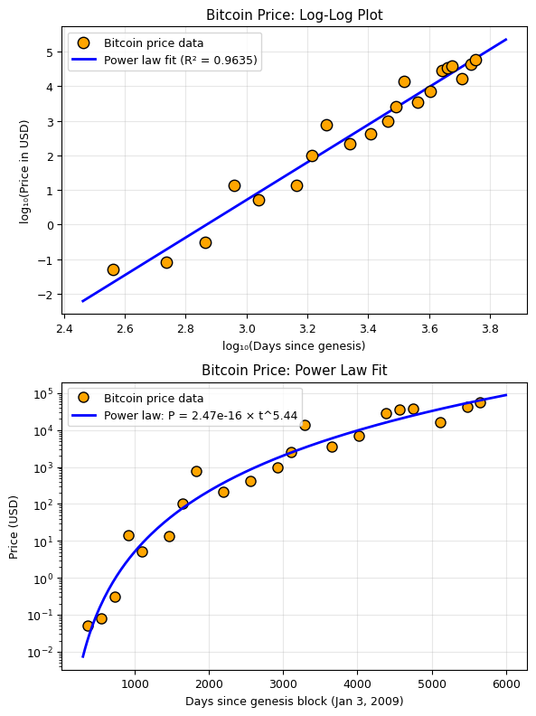
Power law fit (log-log linear regression):
  P(t) = 2.47e-16 × t^5.44
  Exponent n = 5.440
  R² (in log space) = 0.9635

Power law fit (direct curve_fit):
  P(t) = 1.59e-09 × t^3.60

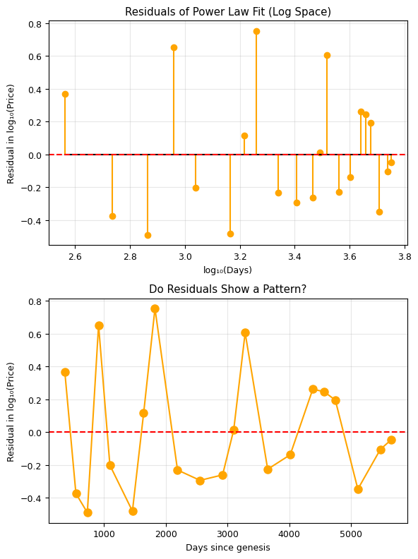
# Critical analysis: examine the residuals in log space
residuals_btc = log_price - np.polyval(p_btc, log_days)

fig, axes = plt.subplots(2, 1, figsize=(6, 8))

# Residuals
axes[0].stem(log_days, residuals_btc, linefmt='orange', markerfmt='o', basefmt='k-')
axes[0].axhline(0, color='r', linestyle='--')
axes[0].set_xlabel('log₁₀(Days)')
axes[0].set_ylabel('Residual in log₁₀(Price)')
axes[0].set_title('Residuals of Power Law Fit (Log Space)')
axes[0].grid(True, alpha=0.3)

# Residuals vs time to check for patterns
axes[1].plot(btc_days, residuals_btc, 'o-', color='orange', markersize=8)
axes[1].axhline(0, color='r', linestyle='--')
axes[1].set_xlabel('Days since genesis')
axes[1].set_ylabel('Residual in log₁₀(Price)')
axes[1].set_title('Do Residuals Show a Pattern?')
axes[1].grid(True, alpha=0.3)

plt.tight_layout()
plt.show()

print('Discussion questions:')
print('1. Do the residuals look random, or is there a pattern (e.g., cycles)?')
print('2. The oscillations around the power law may relate to Bitcoin halving cycles (~4 years)')
print('3. How is this different from Kepler\'s Third Law?')
print('   - Kepler: derived from fundamental physics (gravity)')
print('   - Bitcoin: empirical observation from a complex system (no first-principles derivation)')
print('4. Can we use this fit to PREDICT future prices? Why or why not?')
print('5. What would falsify the power law model?')

Discussion questions:
1. Do the residuals look random, or is there a pattern (e.g., cycles)?
2. The oscillations around the power law may relate to Bitcoin halving cycles (~4 years)
3. How is this different from Kepler's Third Law?
   - Kepler: derived from fundamental physics (gravity)
   - Bitcoin: empirical observation from a complex system (no first-principles derivation)
4. Can we use this fit to PREDICT future prices? Why or why not?
5. What would falsify the power law model?

IX. Advanced Topics (Brief Overview)

Maximum Likelihood Estimation (MLE)

Finds parameters that maximize the probability of observing the data. For Gaussian noise, MLE is equivalent to least squares!

Bayesian Fitting

Uses Bayes’ theorem to compute the posterior probability distribution of parameters:

\[P(\text{params} | \text{data}) \propto P(\text{data} | \text{params}) \times P(\text{params})\]

This gives not just the best parameters, but their full probability distribution!

Weighted Least Squares

When data points have different uncertainties \(\sigma_i\):

\[\text{err} = \sum_i \frac{(y_i - f(x_i))^2}{\sigma_i^2}\]

Points with smaller error bars contribute more to the fit.

# Weighted vs unweighted fitting
np.random.seed(42)
x_w = np.linspace(0, 5, 15)
y_true_w = 2 * x_w + 1

# Different uncertainties: first few points very precise, last few noisy
sigma_w = np.concatenate([0.1 * np.ones(8), 2.0 * np.ones(7)])
y_w = y_true_w + sigma_w * np.random.randn(15)

# Unweighted fit
p_unw = np.polyfit(x_w, y_w, 1)

# Weighted fit
p_weighted = np.polyfit(x_w, y_w, 1, w=1/sigma_w)

plt.figure(figsize=(6, 5))
plt.errorbar(x_w, y_w, yerr=sigma_w, fmt='ko', markersize=6, capsize=5, label='Data')
plt.plot(x_w, np.polyval(p_unw, x_w), 'b-', linewidth=2,
         label=f'Unweighted: y = {p_unw[0]:.2f}x + {p_unw[1]:.2f}')
plt.plot(x_w, np.polyval(p_weighted, x_w), 'r--', linewidth=2,
         label=f'Weighted: y = {p_weighted[0]:.2f}x + {p_weighted[1]:.2f}')
plt.plot(x_w, y_true_w, 'g:', linewidth=2, label='True: y = 2x + 1')
plt.xlabel('x')
plt.ylabel('y')
plt.title('Weighted vs Unweighted Fitting')
plt.legend()
plt.grid(True, alpha=0.3)
plt.tight_layout()
plt.show()

print('Weighted fit trusts precise points more -> closer to true line!')