Lecture 11: Partial Differential Equations (PDEs)

Computational Physics — Spring 2026

Why PDEs?

PDEs describe how quantities vary in both space and time:

Physics	Equation	Type
Heat conduction	\(\partial T/\partial t = \alpha \, \partial^2 T/\partial x^2\)	Parabolic
Wave propagation	\(\partial^2 u/\partial t^2 = c^2 \, \partial^2 u/\partial x^2\)	Hyperbolic
Electrostatics	\(\nabla^2 \phi = -\rho/\epsilon_0\)	Elliptic
Quantum mechanics	\(i\hbar \, \partial\psi/\partial t = -(\hbar^2/2m) \, \partial^2\psi/\partial x^2 + V\psi\)	Parabolic (in imaginary time)
Fluid dynamics	\(\partial \mathbf{v}/\partial t + (\mathbf{v}\cdot\nabla)\mathbf{v} = -\nabla p/\rho + \nu\nabla^2\mathbf{v}\)	Mixed

Strategy: Discretize space on a grid, replace derivatives with finite differences → system of ODEs or algebraic equations.

import numpy as np
import matplotlib.pyplot as plt
from matplotlib import animation
from scipy import sparse
from scipy.sparse.linalg import spsolve

# Projector-friendly settings
plt.rcParams['figure.figsize'] = [6, 4]
plt.rcParams['font.size'] = 9

print("Ready!")

Ready!

I. PDE Classification and Finite Differences

Three Types of PDEs

For a second-order linear PDE \(A u_{xx} + 2B u_{xt} + C u_{tt} = \ldots\) :

Type	Discriminant	Prototype	Physics	Boundary conditions
Parabolic	\(B^2 - AC = 0\)	Heat equation	Diffusion, relaxation	Initial + boundary
Hyperbolic	\(B^2 - AC > 0\)	Wave equation	Waves, vibrations	Initial + boundary
Elliptic	\(B^2 - AC < 0\)	Laplace equation	Steady state, equilibrium	Boundary only

Each type requires different numerical strategies!

Finite Difference Refresher

From Lecture 05, we approximate derivatives on a grid with spacing \(\Delta x\):

\[\frac{\partial u}{\partial x}\bigg|_i \approx \frac{u_{i+1} - u_{i-1}}{2\Delta x}\]

\[\frac{\partial^2 u}{\partial x^2}\bigg|_i \approx \frac{u_{i+1} - 2u_i + u_{i-1}}{\Delta x^2}\]

For time derivatives with spacing \(\Delta t\):

\[\frac{\partial u}{\partial t}\bigg|^n \approx \frac{u^{n+1} - u^n}{\Delta t}\]

Notation: \(u_i^n\) = value at grid point \(i\), time step \(n\).

II. The 1D Heat Equation (Parabolic PDE)

The Physics

A metal rod of length \(L\) with temperature \(T(x, t)\):

\[\frac{\partial T}{\partial t} = \alpha \frac{\partial^2 T}{\partial x^2}\]

where \(\alpha\) is the thermal diffusivity (how fast heat spreads).

FTCS: Forward Time, Central Space

Discretize: forward difference in time, central difference in space:

\[\frac{T_i^{n+1} - T_i^n}{\Delta t} = \alpha \frac{T_{i+1}^n - 2T_i^n + T_{i-1}^n}{\Delta x^2}\]

Solving for the future:

\[\boxed{T_i^{n+1} = T_i^n + r \left(T_{i+1}^n - 2T_i^n + T_{i-1}^n\right)}\]

where \(r = \alpha \Delta t / \Delta x^2\) is the mesh ratio.

def heat_ftcs(T0, alpha, dx, dt, n_steps, bc_left=0.0, bc_right=0.0):
    """Solve the 1D heat equation using FTCS (Forward Time, Central Space).

    Parameters
    ----------
    T0 : ndarray
        Initial temperature profile (N_x points).
    alpha : float
        Thermal diffusivity.
    dx : float
        Spatial grid spacing.
    dt : float
        Time step.
    n_steps : int
        Number of time steps to take.
    bc_left, bc_right : float
        Dirichlet boundary conditions.

    Returns
    -------
    T_history : ndarray
        Temperature at each saved time step, shape (n_saved, N_x).
    """
    N_x = len(T0)
    r = alpha * dt / dx**2   # Mesh ratio

    T = T0.copy()
    save_every = max(1, n_steps // 100)
    T_history = [T.copy()]

    for n in range(n_steps):
        T_new = T.copy()

        # code here
        for i in range(1, N_x -1):
            T_new[i] = T[i] + r*(T[i+1] - 2*T[i] + T[i-1])

        # Apply boundary conditions
        T_new[0] = bc_left
        T_new[-1] = bc_right
        T = T_new
        if (n + 1) % save_every == 0:
            T_history.append(T.copy())

    return np.array(T_history)

# ---- Demo: Hot spot diffusing in a cold rod ----
L = 1.0          # Rod length (m)
N_x = 101        # Grid points
alpha = 0.01     # Thermal diffusivity (m^2/s)
dx = L / (N_x - 1)
x = np.linspace(0, L, N_x)

# Initial condition: Gaussian hot spot in the middle
T0 = np.exp(-((x - 0.5)**2) / (2 * 0.02**2))

# Stable time step (we'll explain why later!)
dt = 0.4 * dx**2 / alpha   # r = 0.4 < 0.5
n_steps = 5000

print(f"Grid spacing: dx = {dx:.4f}")
print(f"Time step:    dt = {dt:.6f}")
print(f"Mesh ratio:   r  = {alpha * dt / dx**2:.2f}")
print(f"Total time:   {n_steps * dt:.2f} s")

T_hist = heat_ftcs(T0, alpha, dx, dt, n_steps)

# Plot snapshots
fig, ax = plt.subplots(figsize=(6, 5))
n_snapshots = min(len(T_hist), 8)
colors = plt.cm.coolwarm(np.linspace(1, 0, n_snapshots))
times = np.linspace(0, n_steps * dt, len(T_hist))

snap_indices = np.linspace(0, len(T_hist)-1, n_snapshots, dtype=int)
for i, idx in enumerate(snap_indices):
    ax.plot(x, T_hist[idx], color=colors[i],
            linewidth=1, label=f't = {times[idx]:.2f} s')

ax.set_xlabel('Position x (m)')
ax.set_ylabel('Temperature T')
ax.set_title('Heat Equation: Gaussian Pulse Diffusing')
ax.legend(fontsize=6, ncol=2)
ax.grid(True, alpha=0.3)
plt.tight_layout()
plt.show()

print("The hot spot spreads out and flattens — diffusion in action!")
print(f"Conservation check: initial integral = {np.trapz(T0, x):.4f}, final = {np.trapz(T_hist[-1], x):.4f}")

Grid spacing: dx = 0.0100
Time step:    dt = 0.004000
Mesh ratio:   r  = 0.40
Total time:   20.00 s

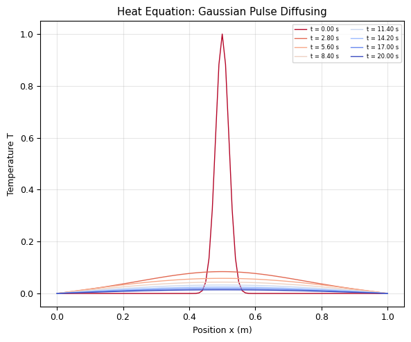
The hot spot spreads out and flattens — diffusion in action!
Conservation check: initial integral = 0.0501, final = 0.0088

/tmp/ipykernel_408/1936641005.py:88: DeprecationWarning: `trapz` is deprecated. Use `trapezoid` instead, or one of the numerical integration functions in `scipy.integrate`.
  print(f"Conservation check: initial integral = {np.trapz(T0, x):.4f}, final = {np.trapz(T_hist[-1], x):.4f}")

III. Stability: Why Your Simulation Can Explode

The CFL Condition

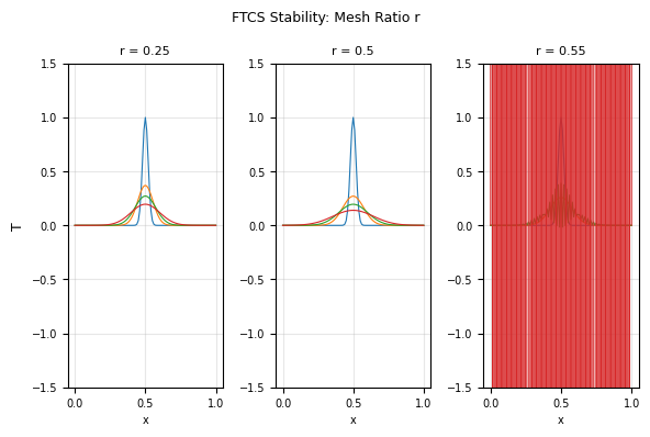
The FTCS scheme is conditionally stable. It only works when:

\[\boxed{r = \frac{\alpha \Delta t}{\Delta x^2} \leq \frac{1}{2}}\]

If \(r > 1/2\), small numerical errors grow exponentially and the solution blows up!

Von Neumann Stability Analysis

Assume a perturbation \(\epsilon_i^n = A^n e^{ijk\Delta x}\). Substituting into the FTCS scheme:

\[A = 1 - 4r\sin^2\!\left(\frac{k\Delta x}{2}\right)\]

For stability, \(|A| \leq 1\) for all \(k\) → the worst case is \(\sin^2 = 1\):

\[|1 - 4r| \leq 1 \quad \Rightarrow \quad r \leq \frac{1}{2}\]

Physical interpretation: Information can’t travel faster than one grid cell per time step.

# Demonstrate instability: r > 0.5
fig, axes = plt.subplots(1, 3, figsize=(6, 4))

for idx, r_val in enumerate([0.25, 0.50, 0.55]):
    dt_test = r_val * dx**2 / alpha
    T_test = heat_ftcs(T0, alpha, dx, dt_test, n_steps=200)

    # Plot a few snapshots
    for snap_idx in [0, len(T_test)//4, len(T_test)//2, -1]:
        axes[idx].plot(x, T_test[snap_idx], linewidth=0.8)

    axes[idx].set_title(f'r = {r_val}', fontsize=8)
    axes[idx].set_xlabel('x', fontsize=7)
    axes[idx].set_ylim(-1.5, 1.5)
    axes[idx].grid(True, alpha=0.3)
    axes[idx].tick_params(labelsize=7)

axes[0].set_ylabel('T')
plt.suptitle('FTCS Stability: Mesh Ratio r', fontsize=9)
plt.tight_layout()
plt.show()

print("r = 0.25: Stable and smooth — diffusion works correctly")
print("r = 0.50: Right at the stability limit — oscillations may appear")
print("r = 0.55: UNSTABLE — oscillations grow exponentially!")
print("This is the CFL condition: Δt ≤ Δx²/(2α)")

r = 0.25: Stable and smooth — diffusion works correctly
r = 0.50: Right at the stability limit — oscillations may appear
r = 0.55: UNSTABLE — oscillations grow exponentially!
This is the CFL condition: Δt ≤ Δx²/(2α)

V. The 1D Wave Equation (Hyperbolic PDE)

The Physics

A vibrating string, sound wave, or electromagnetic wave:

\[\frac{\partial^2 u}{\partial t^2} = c^2 \frac{\partial^2 u}{\partial x^2}\]

Unlike diffusion, waves propagate without spreading — information travels at speed \(c\).

CTCS: Central Time, Central Space

Use central differences in both time and space:

\[\frac{u_i^{n+1} - 2u_i^n + u_i^{n-1}}{\Delta t^2} = c^2 \frac{u_{i+1}^n - 2u_i^n + u_{i-1}^n}{\Delta x^2}\]

Solving for the future:

\[\boxed{u_i^{n+1} = 2u_i^n - u_i^{n-1} + s^2 \left(u_{i+1}^n - 2u_i^n + u_{i-1}^n\right)}\]

where \(s = c \Delta t / \Delta x\) is the Courant number.

Stability (CFL Condition for Waves)

\[s = \frac{c \Delta t}{\Delta x} \leq 1\]

The numerical wave speed must not exceed the physical wave speed.

def wave_ctcs(u0, v0, c, dx, dt, n_steps, bc='fixed'):
    """Solve the 1D wave equation using CTCS (leapfrog) method.

    Parameters
    ----------
    u0 : ndarray
        Initial displacement.
    v0 : ndarray
        Initial velocity.
    c : float
        Wave speed.
    dx, dt : float
        Grid spacing and time step.
    n_steps : int
        Number of time steps.
    bc : str
        'fixed' (Dirichlet u=0) or 'free' (Neumann du/dx=0).

    Returns
    -------
    u_history : ndarray
        Displacement snapshots.
    """
    N = len(u0)
    s = c * dt / dx      # Courant number
    s2 = s**2

    u_prev = u0.copy()
    # First step using initial velocity: u^1 = u^0 + dt*v0 + 0.5*s2*(u_{i+1}-2u_i+u_{i-1})
    u_curr = u0.copy()
    for i in range(1, N-1):
        u_curr[i] = (u0[i] + dt * v0[i]
                     + 0.5 * s2 * (u0[i+1] - 2*u0[i] + u0[i-1]))

    save_every = max(1, n_steps // 200)
    u_history = [u0.copy()]

    for n in range(1, n_steps):
        u_next = np.zeros(N)
        for i in range(1, N-1):
            # u_next[i] =
            u_next[i] = 2*u_curr[i]-u_prev[i] + s2 * (u_curr[i+1] - 2*u_curr[i] + u_curr[i-1])

        # Boundary conditions
        if bc == 'fixed':
            u_next[0] = 0.0
            u_next[-1] = 0.0
        elif bc == 'free':
            u_next[0] = u_next[1]
            u_next[-1] = u_next[-2]

        u_prev = u_curr.copy()
        u_curr = u_next.copy()

        if n % save_every == 0:
            u_history.append(u_curr.copy())

    return np.array(u_history)

# ---- Demo: Plucked string ----
L = 1.0
N_x = 201
c = 1.0        # Wave speed
dx = L / (N_x - 1)
x = np.linspace(0, L, N_x)

# Initial condition: plucked string (triangle)
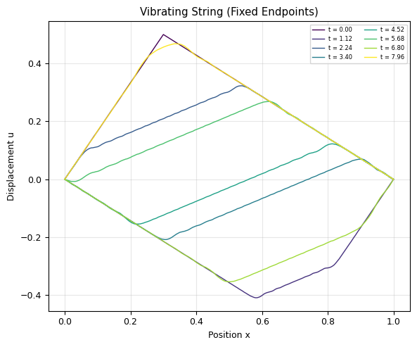
u0 = np.where(x < 0.3, x / 0.3 * 0.5, 0.5 * (1 - x) / 0.7)
u0[0] = 0; u0[-1] = 0   # Fixed endpoints
v0 = np.zeros(N_x)       # Released from rest

# Stable time step
dt = 0.8 * dx / c  # Courant number = 0.8
n_steps = 2000

print(f"Courant number: s = c*dt/dx = {c * dt / dx:.2f}")
print(f"Total simulation time: {n_steps * dt:.2f} s")

u_hist = wave_ctcs(u0, v0, c, dx, dt, n_steps, bc='fixed')

# Plot snapshots
fig, ax = plt.subplots(figsize=(6, 5))
n_show = 8
colors = plt.cm.viridis(np.linspace(0, 1, n_show))

for idx, snap in enumerate(np.linspace(0, len(u_hist)-1, n_show, dtype=int)):
    t_val = snap * (n_steps / len(u_hist)) * dt
    ax.plot(x, u_hist[snap], color=colors[idx], linewidth=1,
            label=f't = {t_val:.2f}')

ax.set_xlabel('Position x')
ax.set_ylabel('Displacement u')
ax.set_title('Vibrating String (Fixed Endpoints)')
ax.legend(fontsize=6, ncol=2)
ax.grid(True, alpha=0.3)
plt.tight_layout()
plt.show()

print("The plucked string vibrates — standing waves form!")
print("Fixed endpoints → only certain wavelengths are allowed (harmonics)")

Courant number: s = c*dt/dx = 0.80
Total simulation time: 8.00 s

The plucked string vibrates — standing waves form!
Fixed endpoints → only certain wavelengths are allowed (harmonics)

Wave Packet Propagation

Let’s watch a Gaussian wave packet travel, reflect off boundaries, and interfere with itself.

# Wave packet: Gaussian envelope * carrier wave
sigma = 0.05
x0_wave = 0.2
k0 = 40.0  # carrier wavevector

u0_packet = np.exp(-((x - x0_wave)**2) / (2*sigma**2)) * np.sin(k0 * x)
u0_packet[0] = 0; u0_packet[-1] = 0
v0_packet = np.zeros(N_x)

dt_wp = 0.9 * dx / c
u_wp = wave_ctcs(u0_packet, v0_packet, c, dx, dt_wp, n_steps=4000, bc='fixed')

# Waterfall plot
fig, ax = plt.subplots(figsize=(6, 6))
n_traces = 30
for idx, snap in enumerate(np.linspace(0, len(u_wp)-1, n_traces, dtype=int)):
    offset = idx * 0.15
    ax.plot(x, u_wp[snap] + offset, 'b-', linewidth=0.5, alpha=0.7)
    ax.fill_between(x, offset, u_wp[snap] + offset, alpha=0.05, color='blue')

ax.set_xlabel('Position x')
ax.set_ylabel('Time →')
ax.set_title('Wave Packet: Propagation & Reflection')
ax.set_yticks([])
plt.tight_layout()
plt.show()

print("The wave packet travels right, reflects off the fixed end (inverted!),")
print("travels left, reflects again, and keeps bouncing.")
print("Fixed boundary: reflection with sign flip (node at boundary)")

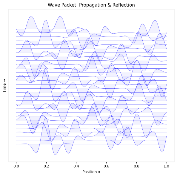
The wave packet travels right, reflects off the fixed end (inverted!),
travels left, reflects again, and keeps bouncing.
Fixed boundary: reflection with sign flip (node at boundary)

VI. The 2D Laplace Equation (Elliptic PDE)

The Physics

In electrostatics, the potential \(\phi\) in a charge-free region satisfies:

\[\nabla^2 \phi = \frac{\partial^2 \phi}{\partial x^2} + \frac{\partial^2 \phi}{\partial y^2} = 0\]

No time variable! This is a boundary value problem — the solution everywhere is determined by the boundary conditions.

Jacobi Relaxation Method

Discretize on a 2D grid. At each interior point:

\[\frac{\phi_{i+1,j} - 2\phi_{i,j} + \phi_{i-1,j}}{\Delta x^2} + \frac{\phi_{i,j+1} - 2\phi_{i,j} + \phi_{i,j-1}}{\Delta y^2} = 0\]

For \(\Delta x = \Delta y\), solve for \(\phi_{i,j}\):

\[\boxed{\phi_{i,j} = \frac{1}{4}\left(\phi_{i+1,j} + \phi_{i-1,j} + \phi_{i,j+1} + \phi_{i,j-1}\right)}\]

Each point is the average of its four neighbors! Iterate until convergence:

1. Initialize with a guess

2. Update every interior point with the 4-neighbor average

3. Check if the solution has changed

4. Repeat until changes are smaller than tolerance

def laplace_jacobi(phi0, bc_mask, max_iter=10000, tol=1e-5):
    """Solve 2D Laplace equation using Jacobi relaxation.

    Parameters
    ----------
    phi0 : ndarray (Ny, Nx)
        Initial guess (including boundary values).
    bc_mask : ndarray of bool (Ny, Nx)
        True where values are fixed (boundary conditions).
    max_iter : int
        Maximum iterations.
    tol : float
        Convergence tolerance (max change per iteration).

    Returns
    -------
    phi : ndarray
        Converged solution.
    residuals : list
        Max residual at each iteration.
    """
    phi = phi0.copy()
    residuals = []

    for iteration in range(max_iter):
        phi_old = phi.copy()

        ## N = len(phi)
        ## for i in range (1, N-1):
        ##.   for j in range (1, N-1):
        ##         phi[i,j] = (phi_old[i-1,j] + phi_old[i+1,j] + phi_old[i,j-1] + phi_old[i,j+1])/4

        # Update interior points: average of 4 neighbors
        phi[1:-1, 1:-1] = 0.25 * (
            phi_old[2:, 1:-1] + phi_old[:-2, 1:-1] +   # up + down
            phi_old[1:-1, 2:] + phi_old[1:-1, :-2]       # right + left
        )

        # Restore boundary conditions
        phi[bc_mask] = phi0[bc_mask]

        # Check convergence
        max_change = np.max(np.abs(phi - phi_old))
        residuals.append(max_change)

        if max_change < tol:
            print(f"Converged in {iteration+1} iterations (max change = {max_change:.2e})")
            break
    else:
        print(f"Warning: did not converge after {max_iter} iterations (max change = {max_change:.2e})")

    return phi, residuals

# ---- Parallel plate capacitor ----
Nx, Ny = 61, 61
phi0 = np.zeros((Ny, Nx))
bc_mask = np.zeros((Ny, Nx), dtype=bool)

# Top plate at y = 0.8, x from 0.2 to 0.8: V = +100
# Bottom plate at y = 0.2, x from 0.2 to 0.8: V = -100
plate_y_top = int(0.8 * (Ny - 1))
plate_y_bot = int(0.2 * (Ny - 1))
plate_x_start = int(0.2 * (Nx - 1))
plate_x_end = int(0.8 * (Nx - 1))

phi0[plate_y_top, plate_x_start:plate_x_end+1] = +100
phi0[plate_y_bot, plate_x_start:plate_x_end+1] = -100
bc_mask[plate_y_top, plate_x_start:plate_x_end+1] = True
bc_mask[plate_y_bot, plate_x_start:plate_x_end+1] = True

# Boundary: walls at V=0
bc_mask[0, :] = True; bc_mask[-1, :] = True
bc_mask[:, 0] = True; bc_mask[:, -1] = True

phi, residuals = laplace_jacobi(phi0, bc_mask, max_iter=20000, tol=1e-6)

# Plot
x_grid = np.linspace(0, 1, Nx)
y_grid = np.linspace(0, 1, Ny)
X, Y = np.meshgrid(x_grid, y_grid)

fig, (ax1, ax2) = plt.subplots(1, 2, figsize=(6, 4))

# Potential contour
cp = ax1.contourf(X, Y, phi, levels=30, cmap='RdBu_r')
ax1.contour(X, Y, phi, levels=15, colors='k', linewidths=0.3)
plt.colorbar(cp, ax=ax1, label='Potential φ (V)')
ax1.set_xlabel('x')
ax1.set_ylabel('y')
ax1.set_title('Electric Potential', fontsize=8)
ax1.set_aspect('equal')

# Electric field (negative gradient of potential)
Ey, Ex = np.gradient(-phi, y_grid, x_grid)
skip = 3
ax2.quiver(X[::skip, ::skip], Y[::skip, ::skip],
           Ex[::skip, ::skip], Ey[::skip, ::skip],
           color='steelblue', scale=2000, width=0.003)
ax2.set_xlabel('x')
ax2.set_ylabel('y')
ax2.set_title('Electric Field E = -∇φ', fontsize=8)
ax2.set_aspect('equal')

plt.suptitle('Parallel Plate Capacitor (Laplace Equation)', fontsize=9)
plt.tight_layout()
plt.show()

print("Between the plates: nearly uniform field (as expected)")
print("Fringe fields visible at the plate edges")

Converged in 1636 iterations (max change = 9.99e-07)

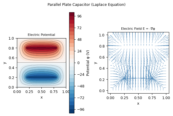
Between the plates: nearly uniform field (as expected)
Fringe fields visible at the plate edges

Convergence of Jacobi Iteration

fig, ax = plt.subplots(figsize=(6, 4))
ax.semilogy(residuals, 'b-', linewidth=0.8)
ax.set_xlabel('Iteration')
ax.set_ylabel('Max change between iterations')
ax.set_title('Jacobi Relaxation Convergence')
ax.axhline(1e-6, color='r', linestyle='--', label='Tolerance = 10⁻⁶')
ax.legend(fontsize=7)
ax.grid(True, alpha=0.3)
plt.tight_layout()
plt.show()

print(f"Jacobi converged in {len(residuals)} iterations.")
print("Gauss-Seidel and SOR (Successive Over-Relaxation) converge faster.")
print("For large problems, multigrid methods are much more efficient.")

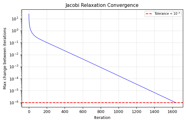
Jacobi converged in 1636 iterations.
Gauss-Seidel and SOR (Successive Over-Relaxation) converge faster.
For large problems, multigrid methods are much more efficient.

VII. Faster Solvers: Gauss-Seidel and SOR

Gauss-Seidel

Same as Jacobi, but use updated values immediately as they become available (just like Euler-Cromer!):

When computing \(\phi_{i,j}\), use the already-updated \(\phi_{i-1,j}\) and \(\phi_{i,j-1}\) from this iteration.

SOR (Successive Over-Relaxation)

Take the Gauss-Seidel update and overshoot:

\[\phi_{i,j}^{\text{new}} = (1-\omega)\,\phi_{i,j}^{\text{old}} + \omega \cdot \frac{1}{4}\left(\phi_{i+1,j} + \phi_{i-1,j} + \phi_{i,j+1} + \phi_{i,j-1}\right)\]

where \(\omega\) is the relaxation parameter:

• \(\omega = 1\): Gauss-Seidel

• \(1 < \omega < 2\): Over-relaxation (faster convergence)

• \(\omega \geq 2\): Unstable!

Optimal \(\omega\) for an \(N \times N\) grid: \(\omega_{\text{opt}} \approx 2 - \frac{2\pi}{N}\)

def laplace_sor(phi0, bc_mask, omega=1.5, max_iter=10000, tol=1e-5):
    """Solve 2D Laplace equation using SOR (Successive Over-Relaxation).

    Parameters
    ----------
    phi0 : ndarray (Ny, Nx)
        Initial guess (including boundary values).
    bc_mask : ndarray of bool
        True where values are fixed.
    omega : float
        Relaxation parameter (1 = Gauss-Seidel, 1 < omega < 2 = SOR).
    max_iter : int
        Maximum iterations.
    tol : float
        Convergence tolerance.

    Returns
    -------
    phi : ndarray
        Converged solution.
    residuals : list
        Max residual at each iteration.
    """
    phi = phi0.copy()
    Ny, Nx = phi.shape
    residuals = []

    for iteration in range(max_iter):
        max_change = 0.0

        for i in range(1, Ny-1):
            for j in range(1, Nx-1):
                if bc_mask[i, j]:
                    continue

                # Gauss-Seidel update (uses already-updated neighbors)
                phi_gs = 0.25 * (phi[i+1, j] + phi[i-1, j] +
                                  phi[i, j+1] + phi[i, j-1])

                # SOR: blend old and Gauss-Seidel
                phi_new = (1 - omega) * phi[i, j] + omega * phi_gs

                change = abs(phi_new - phi[i, j])
                if change > max_change:
                    max_change = change
                phi[i, j] = phi_new

        residuals.append(max_change)
        if max_change < tol:
            break

    return phi, residuals

# Compare Jacobi vs Gauss-Seidel vs SOR
omega_opt = 2 - 2*np.pi / Nx  # Optimal relaxation parameter

print(f"Grid size: {Nx}x{Ny}")
print(f"Optimal ω ≈ {omega_opt:.3f}")
print()

_, res_jacobi = laplace_jacobi(phi0, bc_mask, max_iter=20000, tol=1e-6)
_, res_gs = laplace_sor(phi0, bc_mask, omega=1.0, max_iter=20000, tol=1e-6)
_, res_sor = laplace_sor(phi0, bc_mask, omega=omega_opt, max_iter=20000, tol=1e-6)

fig, ax = plt.subplots(figsize=(6, 4))
ax.semilogy(res_jacobi, 'r-', linewidth=0.8, label=f'Jacobi ({len(res_jacobi)} iter)')
ax.semilogy(res_gs, 'b-', linewidth=0.8, label=f'Gauss-Seidel ({len(res_gs)} iter)')
ax.semilogy(res_sor, 'g-', linewidth=0.8, label=f'SOR ω={omega_opt:.2f} ({len(res_sor)} iter)')
ax.axhline(1e-6, color='k', linestyle='--', alpha=0.5)
ax.set_xlabel('Iteration')
ax.set_ylabel('Max change')
ax.set_title('Convergence: Jacobi vs Gauss-Seidel vs SOR')
ax.legend(fontsize=7)
ax.grid(True, alpha=0.3)
plt.tight_layout()
plt.show()

print(f"Jacobi:       {len(res_jacobi)} iterations")
print(f"Gauss-Seidel: {len(res_gs)} iterations ({len(res_jacobi)/len(res_gs):.1f}x faster)")
print(f"SOR:          {len(res_sor)} iterations ({len(res_jacobi)/len(res_sor):.1f}x faster)")

Grid size: 61x61
Optimal ω ≈ 1.897

Converged in 1636 iterations (max change = 9.99e-07)

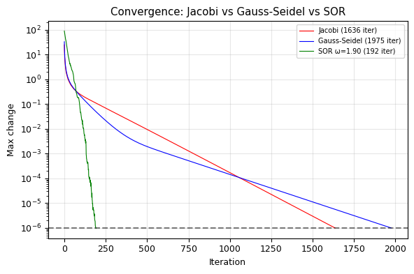
Jacobi:       1636 iterations
Gauss-Seidel: 1975 iterations (0.8x faster)
SOR:          192 iterations (8.5x faster)

VIII. Physics Application: Poisson Equation (Charges!)

The Poisson equation includes a source term:

\[\nabla^2 \phi = -\frac{\rho}{\epsilon_0}\]

This describes the electric potential from a charge distribution \(\rho(x, y)\).

We modify the Jacobi update:

\[\phi_{i,j} = \frac{1}{4}\left(\phi_{i+1,j} + \phi_{i-1,j} + \phi_{i,j+1} + \phi_{i,j-1}\right) + \frac{\Delta x^2}{4\epsilon_0} \rho_{i,j}\]

def poisson_jacobi(phi0, rho, bc_mask, dx, epsilon_0=1.0, max_iter=20000, tol=1e-5):
    """Solve 2D Poisson equation using Jacobi iteration.

    ∇²φ = -ρ/ε₀
    """
    phi = phi0.copy()
    source = (dx**2 / (4 * epsilon_0)) * rho
    residuals = []

    for iteration in range(max_iter):
        phi_old = phi.copy()
        phi[1:-1, 1:-1] = 0.25 * (
            phi_old[2:, 1:-1] + phi_old[:-2, 1:-1] +
            phi_old[1:-1, 2:] + phi_old[1:-1, :-2]
        ) + source[1:-1, 1:-1]

        phi[bc_mask] = phi0[bc_mask]

        max_change = np.max(np.abs(phi - phi_old))
        residuals.append(max_change)
        if max_change < tol:
            print(f"Converged in {iteration+1} iterations")
            break

    return phi, residuals

# ---- Electric dipole ----
Nx2, Ny2 = 81, 81
dx2 = 1.0 / (Nx2 - 1)
x2 = np.linspace(0, 1, Nx2)
y2 = np.linspace(0, 1, Ny2)
X2, Y2 = np.meshgrid(x2, y2)

# Charge distribution: +Q and -Q
rho = np.zeros((Ny2, Nx2))
# Positive charge at (0.35, 0.5)
q_plus_j = int(0.35 * (Nx2 - 1))
q_plus_i = int(0.5 * (Ny2 - 1))
rho[q_plus_i, q_plus_j] = +1000 / dx2**2

# Negative charge at (0.65, 0.5)
q_minus_j = int(0.65 * (Nx2 - 1))
q_minus_i = int(0.5 * (Ny2 - 1))
rho[q_minus_i, q_minus_j] = -1000 / dx2**2

# Boundary: grounded box (φ = 0)
phi0_poisson = np.zeros((Ny2, Nx2))
bc_mask2 = np.zeros((Ny2, Nx2), dtype=bool)
bc_mask2[0, :] = True; bc_mask2[-1, :] = True
bc_mask2[:, 0] = True; bc_mask2[:, -1] = True

phi_dipole, _ = poisson_jacobi(phi0_poisson, rho, bc_mask2, dx2, max_iter=30000, tol=1e-5)

# Plot
fig, (ax1, ax2) = plt.subplots(1, 2, figsize=(6, 4))

# Potential
levels = np.linspace(-50, 50, 31)
cp = ax1.contourf(X2, Y2, phi_dipole, levels=levels, cmap='RdBu_r', extend='both')
ax1.contour(X2, Y2, phi_dipole, levels=levels[::2], colors='k', linewidths=0.2)
plt.colorbar(cp, ax=ax1, label='φ')
ax1.plot(x2[q_plus_j], y2[q_plus_i], 'r+', markersize=12, markeredgewidth=2)
ax1.plot(x2[q_minus_j], y2[q_minus_i], 'b_', markersize=12, markeredgewidth=2)
ax1.set_title('Potential (dipole)', fontsize=8)
ax1.set_aspect('equal')
ax1.set_xlabel('x'); ax1.set_ylabel('y')

# Electric field
Ey2, Ex2 = np.gradient(-phi_dipole, y2, x2)
E_mag = np.sqrt(Ex2**2 + Ey2**2)
skip2 = 4
ax2.streamplot(X2, Y2, Ex2, Ey2, color=np.log10(E_mag + 1),
               cmap='hot', density=1.5, linewidth=0.5, arrowsize=0.5)
ax2.plot(x2[q_plus_j], y2[q_plus_i], 'r+', markersize=12, markeredgewidth=2, label='+Q')
ax2.plot(x2[q_minus_j], y2[q_minus_i], 'b_', markersize=12, markeredgewidth=2, label='-Q')
ax2.set_title('Electric Field Lines', fontsize=8)
ax2.set_aspect('equal')
ax2.set_xlabel('x'); ax2.set_ylabel('y')
ax2.legend(fontsize=7)

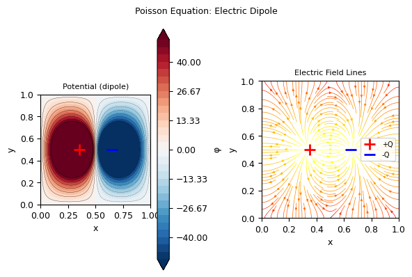
plt.suptitle('Poisson Equation: Electric Dipole', fontsize=9)
plt.tight_layout()
plt.show()

print("Field lines go from + to - charge")
print("Equipotential lines (contours) are perpendicular to field lines")
print("Far from the dipole: field falls off as 1/r³")

Converged in 5617 iterations

Field lines go from + to - charge
Equipotential lines (contours) are perpendicular to field lines
Far from the dipole: field falls off as 1/r³

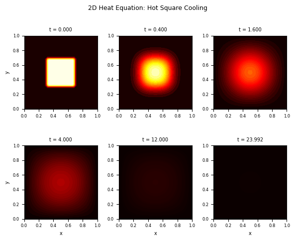
IX. Physics Application: 2D Heat Equation

Combining spatial dimensions:

\[\frac{\partial T}{\partial t} = \alpha\left(\frac{\partial^2 T}{\partial x^2} + \frac{\partial^2 T}{\partial y^2}\right)\]

FTCS in 2D:

\[T_{i,j}^{n+1} = T_{i,j}^n + r_x(T_{i+1,j}^n - 2T_{i,j}^n + T_{i-1,j}^n) + r_y(T_{i,j+1}^n - 2T_{i,j}^n + T_{i,j-1}^n)\]

Stability requires: \(r_x + r_y \leq 1/2\) where \(r_x = \alpha\Delta t/\Delta x^2\), \(r_y = \alpha\Delta t/\Delta y^2\).

# 2D heat equation: hot square cooling into cold plate
Nx3 = 51
Ny3 = 51
alpha_2d = 0.01
dx3 = 1.0 / (Nx3 - 1)
dy3 = 1.0 / (Ny3 - 1)
x3 = np.linspace(0, 1, Nx3)
y3 = np.linspace(0, 1, Ny3)
X3, Y3 = np.meshgrid(x3, y3)

# Initial condition: hot square in center
T2d = np.zeros((Ny3, Nx3))
hot_region = (X3 > 0.3) & (X3 < 0.7) & (Y3 > 0.3) & (Y3 < 0.7)
T2d[hot_region] = 100.0

# Stable time step
dt3 = 0.2 * dx3**2 / alpha_2d  # conservative for 2D
rx = alpha_2d * dt3 / dx3**2
ry = alpha_2d * dt3 / dy3**2
print(f"rx + ry = {rx + ry:.3f} (must be ≤ 0.5)")

# Time-stepping
n_steps_2d = 3000
snapshots = []
snap_times = []

T = T2d.copy()
for n in range(n_steps_2d):
    T_new = T.copy()
    T_new[1:-1, 1:-1] = T[1:-1, 1:-1] + (
        rx * (T[2:, 1:-1] - 2*T[1:-1, 1:-1] + T[:-2, 1:-1]) +
        ry * (T[1:-1, 2:] - 2*T[1:-1, 1:-1] + T[1:-1, :-2])
    )
    # Dirichlet BC: T = 0 on all boundaries
    T_new[0, :] = 0; T_new[-1, :] = 0
    T_new[:, 0] = 0; T_new[:, -1] = 0
    T = T_new

    if n in [0, 50, 200, 500, 1500, n_steps_2d-1]:
        snapshots.append(T.copy())
        snap_times.append(n * dt3)

# Plot
fig, axes = plt.subplots(2, 3, figsize=(6, 5))
axes = axes.flatten()

for idx, (snap, t_val) in enumerate(zip(snapshots, snap_times)):
    im = axes[idx].contourf(X3, Y3, snap, levels=20, cmap='hot', vmin=0, vmax=100)
    axes[idx].set_title(f't = {t_val:.3f}', fontsize=7)
    axes[idx].set_aspect('equal')
    axes[idx].tick_params(labelsize=6)
    if idx % 3 == 0:
        axes[idx].set_ylabel('y', fontsize=7)
    if idx >= 3:
        axes[idx].set_xlabel('x', fontsize=7)

plt.suptitle('2D Heat Equation: Hot Square Cooling', fontsize=9)
plt.tight_layout()
plt.show()

print("The sharp edges smooth out first (high curvature → fast diffusion)")
print("Eventually the temperature decays to zero everywhere")
print(f"Total heat: initial = {np.sum(T2d)*dx3*dy3:.2f}, final = {np.sum(snapshots[-1])*dx3*dy3:.2f}")

rx + ry = 0.400 (must be ≤ 0.5)

The sharp edges smooth out first (high curvature → fast diffusion)
Eventually the temperature decays to zero everywhere
Total heat: initial = 14.44, final = 0.18

X. Solving PDEs with FFT: Spectral Methods

All the methods above use finite differences — local approximations to derivatives. There’s a completely different approach that uses the FFT from Lecture 09.

The Key Insight: Derivatives Become Multiplication

Recall from Fourier analysis that the Fourier transform turns derivatives into algebraic operations:

\[\mathcal{F}\left\{\frac{\partial f}{\partial x}\right\} = i k \, \hat{f}(k)\]

\[\mathcal{F}\left\{\frac{\partial^2 f}{\partial x^2}\right\} = (ik)^2 \, \hat{f}(k) = -k^2 \, \hat{f}(k)\]

where \(k\) is the wavenumber and \(\hat{f}(k)\) is the Fourier transform of \(f(x)\).

This means we can compute spatial derivatives exactly (to machine precision!) by:

1. FFT the function: \(f(x) \to \hat{f}(k)\)

2. Multiply by \(-k^2\): \(\hat{f}(k) \to -k^2\,\hat{f}(k)\)

3. Inverse FFT: \(-k^2\,\hat{f}(k) \to f''(x)\)

No finite difference approximation needed!

Application to the Heat Equation

Take the heat equation \(\partial T/\partial t = \alpha \, \partial^2 T/\partial x^2\) and Fourier-transform in space:

\[\frac{\partial \hat{T}(k,t)}{\partial t} = -\alpha k^2 \, \hat{T}(k,t)\]

This is now an ODE for each wavenumber \(k\) — and it has an exact solution:

\[\hat{T}(k, t) = \hat{T}(k, 0) \, e^{-\alpha k^2 t}\]

Algorithm (analytical spectral method):

1. FFT the initial condition: \(T(x,0) \to \hat{T}(k,0)\)

2. Multiply each mode by the decay factor: \(\hat{T}(k,0) \cdot e^{-\alpha k^2 t}\)

3. Inverse FFT to get \(T(x, t)\)

No time stepping at all! We jump directly to any future time.

Why Spectral Methods Are Special

Property	Finite Difference	Spectral (FFT)
Spatial accuracy	\(O(\Delta x^2)\)	Exponential (machine precision for smooth functions)
Stability limit	CFL: \(r \leq 1/2\)	None (analytical solution)
Boundary conditions	Any (Dirichlet, Neumann, …)	Periodic only (limitation!)
Cost per step	\(O(N)\)	\(O(N \log N)\)
Best for	General geometries, non-periodic BC	Smooth periodic problems, turbulence

Limitation: The standard FFT assumes periodic boundary conditions. For non-periodic problems, you need basis functions other than \(e^{ikx}\) — e.g., Chebyshev polynomials (Chebyshev spectral methods).

Spectral Time-Stepping (for more general PDEs)

When you can’t solve analytically (e.g., nonlinear PDEs), use the FFT just for spatial derivatives:

1. Compute \(\partial^2 T/\partial x^2\) spectrally: FFT → multiply by -k² → IFFT

2. Time-step with any ODE method (Euler, RK4, etc.)

This gives spectral accuracy in space with your choice of time integrator.

# ---- Spectral Method for the Heat Equation ----
# Compare: FTCS (finite difference) vs Spectral (FFT)

# Setup: periodic domain [0, L) with Gaussian initial condition
L_sp = 2.0
N_sp = 128          # Grid points (power of 2 for FFT efficiency)
alpha_sp = 0.01     # Thermal diffusivity
dx_sp = L_sp / N_sp
x_sp = np.linspace(0, L_sp, N_sp, endpoint=False)  # Periodic: no repeated endpoint

# Initial condition: Gaussian (periodic-compatible)
T0_sp = np.exp(-((x_sp - 1.0)**2) / (2 * 0.05**2))

# ---- Method 1: Analytical spectral solution ----
# Wavenumbers for FFT (numpy convention)
k = 2 * np.pi * np.fft.fftfreq(N_sp, d=dx_sp)

# FFT of initial condition
T0_hat = np.fft.fft(T0_sp)

# Solve at multiple times — NO time stepping needed!
t_targets = [0, 0.5, 1.0, 2.0, 5.0]

fig, (ax1, ax2) = plt.subplots(1, 2, figsize=(6, 4))

colors_sp = plt.cm.coolwarm(np.linspace(1, 0, len(t_targets)))
for idx, t_val in enumerate(t_targets):
    # Exact spectral solution: multiply each mode by exp(-α k² t)
    decay = np.exp(-alpha_sp * k**2 * t_val)
    T_hat_t = T0_hat * decay
    T_spectral = np.real(np.fft.ifft(T_hat_t))
    ax1.plot(x_sp, T_spectral, color=colors_sp[idx], linewidth=1,
             label=f't = {t_val}')

ax1.set_xlabel('x')
ax1.set_ylabel('T')
ax1.set_title('Spectral Method (exact!)', fontsize=8)
ax1.legend(fontsize=6)
ax1.grid(True, alpha=0.3)

# ---- Show the decay of Fourier modes ----
k_pos = k[:N_sp//2]
for t_val in [0, 0.5, 2.0, 5.0]:
    decay = np.exp(-alpha_sp * k_pos**2 * t_val)
    ax2.plot(k_pos, decay, linewidth=1, label=f't = {t_val}')

ax2.set_xlabel('Wavenumber k')
ax2.set_ylabel('Decay factor $e^{-\\alpha k^2 t}$')
ax2.set_title('High-k modes decay fastest', fontsize=8)
ax2.legend(fontsize=6)
ax2.grid(True, alpha=0.3)

plt.suptitle('FFT Spectral Method: Heat Equation', fontsize=9)
plt.tight_layout()
plt.show()

print("Spectral method: NO time stepping, NO stability limit!")
print("We jump directly to any time t by multiplying Fourier modes by exp(-αk²t).")
print("High-frequency modes (large k) decay fastest — that's why diffusion smooths things out.")

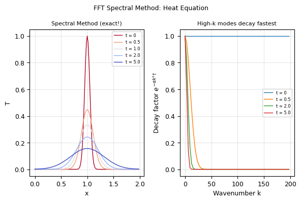
Spectral method: NO time stepping, NO stability limit!
We jump directly to any time t by multiplying Fourier modes by exp(-αk²t).
High-frequency modes (large k) decay fastest — that's why diffusion smooths things out.