Lecture 15: Optimization I — Gradient Descent and Line Search#
Computational Physics — Spring 2026
Finding Minima: The Core Problem of Computational Science#
Optimization is one of the most fundamental tasks in computational physics. Nearly every simulation, fit, or model ultimately requires finding the minimum of some function:
Molecular physics: Finding stable configurations (minimize potential energy)
Data fitting: Minimizing the residual between model and data (Lecture 7, HW4)
Quantum mechanics: Variational principle — the ground state minimizes \(\langle \hat{H} \rangle\) (Lecture 13 VMC)
Machine learning: Training = minimizing a loss function
In Lecture 14, we used simulated annealing — a global, stochastic optimizer. Today we study local optimization: deterministic methods that follow the landscape downhill to the nearest minimum.
Today’s roadmap:
The optimization landscape: local vs global minima
1D gradient descent: fixed step and adaptive step
Golden section search: derivative-free 1D optimization
Extending gradient descent to 2D
Introduction to
scipy.optimize
import numpy as np
import matplotlib.pyplot as plt

plt.rcParams['figure.figsize'] = [6, 4]
plt.rcParams['font.size'] = 9

print("Ready for optimization!")
Ready for optimization!
I. The Optimization Landscape#
Local vs Global Minima#
Given a function \(f(x)\), we want to find \(x^*\) such that \(f(x^*) \leq f(x)\) for all \(x\) nearby.
Key concepts:
Local minimum: \(f(x^*) \leq f(x)\) for all \(x\) in a neighborhood of \(x^*\)
Global minimum: \(f(x^*) \leq f(x)\) for all \(x\)
Saddle point: A point where the gradient is zero but it’s neither a minimum nor maximum
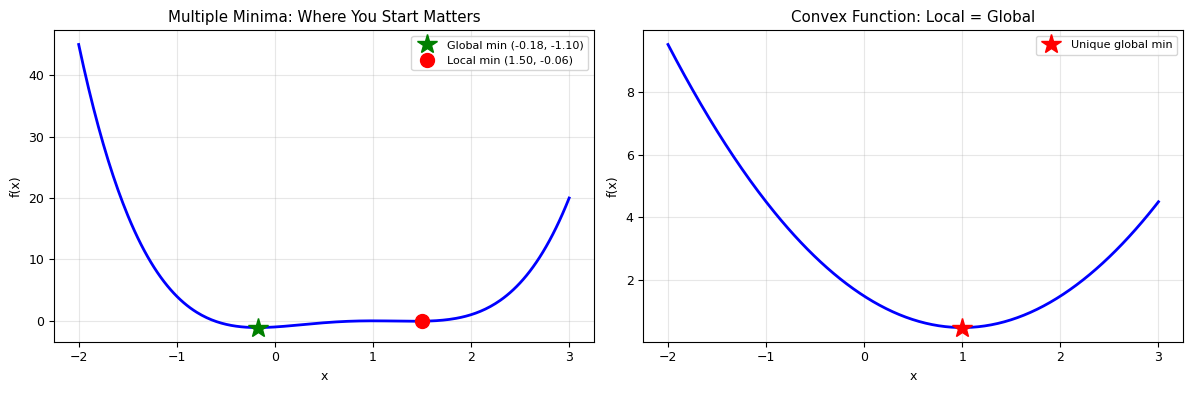
Convex function: A function where every local minimum is also the global minimum
Necessary condition for a minimum: \(f'(x^*) = 0\) and \(f''(x^*) > 0\).
The challenge: Local optimization methods can only find local minima. The result depends on where we start. This is why we ran simulated annealing in Lecture 14 — it can escape local minima via thermal fluctuations.
# Visualize: a landscape with multiple minima
x = np.linspace(-2, 3, 300)
f_landscape = lambda x: x**4 - 3*x**3 + 2*x**2 + x - 1

fig, axes = plt.subplots(1, 2, figsize=(12, 4))

# Left: function with local and global minima
axes[0].plot(x, f_landscape(x), 'b-', lw=2)
axes[0].set_xlabel('x')
axes[0].set_ylabel('f(x)')
axes[0].set_title('Multiple Minima: Where You Start Matters')
axes[0].grid(alpha=0.3)

# Mark local and global minima (approximate)
from scipy.optimize import minimize_scalar
res1 = minimize_scalar(f_landscape, bounds=(-1, 0.5), method='bounded')
res2 = minimize_scalar(f_landscape, bounds=(1.5, 3), method='bounded')
axes[0].plot(res1.x, res1.fun, 'g*', ms=15, label=f'Global min ({res1.x:.2f}, {res1.fun:.2f})')
axes[0].plot(res2.x, res2.fun, 'ro', ms=10, label=f'Local min ({res2.x:.2f}, {res2.fun:.2f})')
axes[0].legend(fontsize=8)

# Right: convex function — every local min is global
f_convex = lambda x: (x - 1)**2 + 0.5
axes[1].plot(x, f_convex(x), 'b-', lw=2)
axes[1].plot(1, 0.5, 'r*', ms=15, label='Unique global min')
axes[1].set_xlabel('x')
axes[1].set_ylabel('f(x)')
axes[1].set_title('Convex Function: Local = Global')
axes[1].legend(fontsize=8)
axes[1].grid(alpha=0.3)

plt.tight_layout()
plt.show()

print("For convex functions, any local minimum is the global minimum.")
print("For non-convex functions, the result depends on the starting point!")
For convex functions, any local minimum is the global minimum.
For non-convex functions, the result depends on the starting point!
II. 1D Optimization: Gradient Descent#
The Gradient Descent Algorithm#
The simplest optimization method: follow the slope downhill.
Update rule:
where \(\eta\) is the step size (or learning rate).
If \(f'(x_n) > 0\): the function is increasing, so we move left (\(x\) decreases)
If \(f'(x_n) < 0\): the function is decreasing, so we move right (\(x\) increases)
If \(f'(x_n) = 0\): we’re at a critical point (minimum, maximum, or saddle)
We approximate the derivative numerically using the central difference formula:
Why Step Size Matters#
\(\eta\) too large: overshoot the minimum, oscillate or diverge
\(\eta\) too small: converge very slowly, waste computation
Just right: efficient convergence
Test Function: A Cubic Polynomial#
with \(A = 1.2\), \(B = 3.0\), \(C = 0.6\). This function has a local minimum near \(x = 0\) and goes to \(-\infty\) as \(x \to -\infty\).
# Define coefficients for our polynomial
A, B, C = 1.2, 3.0, 0.6

x_min, x_max = -1, 1
f = lambda x: A*x**3 + B*x**2 + C

# Visualize
x = np.linspace(x_min, x_max, 101)
plt.figure(figsize=(8, 4))
plt.plot(x, f(x), 'b-', lw=2, label='$f(x) = 1.2x^3 + 3x^2 + 0.6$')
plt.xlabel('x')
plt.ylabel('f(x)')
plt.title('Our Test Function')
plt.legend()
plt.grid(alpha=0.3)
plt.show()

# Analytical minimum: f'(x) = 3Ax^2 + 2Bx = 0 => x = 0 or x = -2B/(3A)
x_crit = -2*B / (3*A)
print(f"Critical points: x = 0 and x = {x_crit:.4f}")
print(f"f(0) = {f(0):.4f}, f({x_crit:.4f}) = {f(x_crit):.4f}")
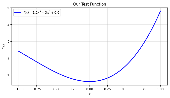
Critical points: x = 0 and x = -1.6667
f(0) = 0.6000, f(-1.6667) = 3.3778
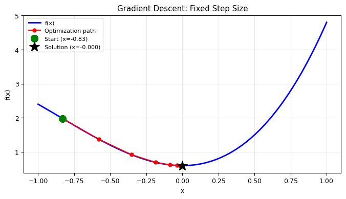
Implementation: Fixed Step Size#
def derivative(f, x, dx=0.01):
    """Numerical derivative using central difference."""
    return (f(x + dx) - f(x - dx)) / (2 * dx)

def minimize(f, x0, dx=0.01, N=1000):
    """Gradient descent with fixed step size.

    Args:
        f: function to minimize
        x0: starting point
        dx: step size (learning rate)
        N: max iterations

    Returns:
        converged, x_best, f_min, x_hist, step
    """
    x_now = x0
    converged = False
    x_hist = [x0]

    for i in range(N):
        x_next = x_now - dx * derivative(f, x_now)
        if f(x_next) < f(x_now):
            x_now = x_next
            x_hist.append(x_now)
        else:
            converged = True
            break

    step = i
    return converged, x_now, f(x_now), np.array(x_hist), step
# Test with a specific starting point
x0 = -0.83
converged, x_best, f_min, x_hist, step = minimize(f, x0, dx=0.1)

print(f'Starting point: x0 = {x0}')
print(f'Converged: {converged}')
print(f'Best solution: x = {x_best:.4f}, f = {f_min:.4f}')
print(f'Steps taken: {step}')

# Visualize the optimization path
x = np.linspace(x_min, x_max, 101)
plt.figure(figsize=(8, 4))
plt.plot(x, f(x), 'b-', lw=2, label='f(x)')
plt.plot(x_hist, f(x_hist), 'ro-', ms=5, label='Optimization path')
plt.plot(x0, f(x0), 'go', ms=10, label=f'Start (x={x0})')
plt.plot(x_best, f_min, 'k*', ms=15, label=f'Solution (x={x_best:.3f})')
plt.xlabel('x')
plt.ylabel('f(x)')
plt.title('Gradient Descent: Fixed Step Size')
plt.legend(fontsize=8)
plt.grid(alpha=0.3)
plt.show()
Starting point: x0 = -0.83
Converged: True
Best solution: x = -0.0000, f = 0.6000
Steps taken: 33
Sensitivity to Starting Point#
Let’s run many trials with random starting points to see how the result depends on where we begin.
np.random.seed(42)

print(f'{"x0":>10s} | {"Converged":>9s} | {"x_best":>8s} | {"f(x_best)":>10s} | {"Steps":>5s}')
print('-' * 55)

for i in range(20):
    x1 = x_min + np.random.random() * (x_max - x_min)
    converged, x_best, f_min, x_hist, step = minimize(f, x1, dx=0.02)
    print(f'{x1:10.4f} | {str(converged):>9s} | {x_best:8.4f} | {f_min:10.4f} | {step:5d}')
        x0 | Converged |   x_best |  f(x_best) | Steps
-------------------------------------------------------
   -0.2509 |      True |  -0.0000 |     0.6000 |   193
    0.9014 |      True |  -0.0000 |     0.6000 |    80
    0.4640 |      True |   0.0000 |     0.6000 |    76
    0.1973 |      True |  -0.0000 |     0.6000 |    71
   -0.6880 |      True |  -0.0000 |     0.6000 |   204
   -0.6880 |      True |  -0.0000 |     0.6000 |   204
   -0.8838 |      True |  -0.0000 |     0.6000 |   208
    0.7324 |      True |  -0.0000 |     0.6000 |    79
    0.2022 |      True |   0.0000 |     0.6000 |    71
    0.4161 |      True |  -0.0000 |     0.6000 |    76
   -0.9588 |      True |  -0.0000 |     0.6000 |   211
    0.9398 |      True |   0.0000 |     0.6000 |    80
    0.6649 |      True |   0.0000 |     0.6000 |    78
   -0.5753 |      True |  -0.0000 |     0.6000 |   203
   -0.6364 |      True |  -0.0000 |     0.6000 |   203
   -0.6332 |      True |  -0.0000 |     0.6000 |   203
   -0.3915 |      True |  -0.0000 |     0.6000 |   199
    0.0495 |      True |  -0.0000 |     0.6000 |    61
   -0.1361 |      True |  -0.0000 |     0.6000 |   189
   -0.4175 |      True |  -0.0000 |     0.6000 |   198
Improvement: Variable Step Size (Barzilai-Borwein Method)#
Instead of a fixed \(\eta\), we can adapt the step size at each iteration. The Barzilai-Borwein method uses information from the previous step:
This is derived from a secant approximation to the Hessian. The idea: if the gradient hasn’t changed much, take a larger step; if it changed a lot, take a smaller step.
def minimize2(f, x0, N=1000):
    """Gradient descent with Barzilai-Borwein variable step size."""
    x_now = x0
    x_prev = None
    converged = False
    x_hist = [x0]

    dx = 0.1  # initial step size
    for i in range(N):
        if x_prev is not None:
            dfx = derivative(f, x_now) - derivative(f, x_prev)
            if abs(dfx) > 1e-8:
                dx = (x_now - x_prev) / dfx
            else:
                dx = 0.1

        x_next = x_now - derivative(f, x_now) * dx
        if f(x_next) < f(x_now):
            x_prev = x_now
            x_now = x_next
            x_hist.append(x_now)
        else:
            converged = True
            break

    return converged, x_now, f(x_now), np.array(x_hist), i

# Compare with fixed step
np.random.seed(42)
print(f'{"x0":>10s} | {"Method":>10s} | {"Converged":>9s} | {"x_best":>8s} | {"f(x_best)":>10s} | {"Steps":>5s}')
print('-' * 70)

for i in range(10):
    x1 = x_min + np.random.random() * (x_max - x_min)
    c1, xb1, fm1, _, s1 = minimize(f, x1, dx=0.05)
    c2, xb2, fm2, _, s2 = minimize2(f, x1)
    print(f'{x1:10.4f} | {"Fixed":>10s} | {str(c1):>9s} | {xb1:8.4f} | {fm1:10.4f} | {s1:5d}')
    print(f'{"":>10s} | {"Variable":>10s} | {str(c2):>9s} | {xb2:8.4f} | {fm2:10.4f} | {s2:5d}')
    print()
        x0 |     Method | Converged |   x_best |  f(x_best) | Steps
----------------------------------------------------------------------
   -0.2509 |      Fixed |      True |  -0.0000 |     0.6000 |    72
           |   Variable |      True |  -0.0000 |     0.6000 |     5

    0.9014 |      Fixed |      True |   0.0000 |     0.6000 |    28
           |   Variable |      True |  -0.0000 |     0.6000 |     4

    0.4640 |      Fixed |      True |   0.0000 |     0.6000 |    27
           |   Variable |      True |  -0.0000 |     0.6000 |     4

    0.1973 |      Fixed |      True |   0.0000 |     0.6000 |    25
           |   Variable |      True |  -0.0000 |     0.6000 |     4

   -0.6880 |      Fixed |      True |  -0.0000 |     0.6000 |    78
           |   Variable |      True |  -0.4456 |     1.0895 |     1

   -0.6880 |      Fixed |      True |  -0.0000 |     0.6000 |    78
           |   Variable |      True |  -0.4456 |     1.0896 |     1

   -0.8838 |      Fixed |      True |  -0.0000 |     0.6000 |    78
           |   Variable |      True |  -0.6348 |     1.5019 |     1

    0.7324 |      Fixed |      True |  -0.0000 |     0.6000 |    28
           |   Variable |      True |   0.0000 |     0.6000 |     4

    0.2022 |      Fixed |      True |   0.0000 |     0.6000 |    25
           |   Variable |      True |  -0.0000 |     0.6000 |     4

    0.4161 |      Fixed |      True |  -0.0000 |     0.6000 |    27
           |   Variable |      True |  -0.0000 |     0.6000 |     4
III. Golden Section Search: No Derivatives Needed#
A Different Approach: Bracket-Based Search#
Gradient descent requires computing \(f'(x)\). What if the derivative is expensive or doesn’t exist? We can use a bracketing method instead.
Idea: Maintain a bracket \([a, b]\) that contains the minimum, and shrink it at each step.
The Golden Section Search#
Analogous to the bisection method for root-finding, but for minimization.
Algorithm:
Start with bracket \([a, b]\) containing a minimum
Evaluate \(f\) at two interior points: $\(x_1 = a + (1 - \varphi)(b - a), \quad x_2 = a + \varphi(b - a)\)\( where \)\varphi = \frac{\sqrt{5} - 1}{2} \approx 0.618$ is the golden ratio conjugate
If \(f(x_1) < f(x_2)\): the minimum is in \([a, x_2]\) — set \(b = x_2\)
If \(f(x_1) \geq f(x_2)\): the minimum is in \([x_1, b]\) — set \(a = x_1\)
Repeat until \(|b - a| < \text{tolerance}\)
Why the Golden Ratio?#
The key insight: with the golden ratio, one of the two evaluation points from the previous step can be reused in the next step. This means we only need one new function evaluation per step (instead of two), cutting the work in half.
Proof: After narrowing \([a, b]\) to \([a, x_2]\), the old point \(x_1\) satisfies:
So \(x_1\) is at position \(\varphi\) within \([a, x_2]\) — exactly where the new upper evaluation point should be! This works because \(\varphi\) satisfies \(\varphi^2 + \varphi = 1\), the defining property of the golden ratio. \(\square\)
Convergence: The bracket shrinks by factor \(\varphi \approx 0.618\) at each step, giving linear convergence.
def golden_section_search(f, a, b, tol=1e-6, N=100):
    """Golden section search for minimum of f on [a, b].

    Requires: f has a single minimum in [a, b] (unimodal).
    """
    phi = (np.sqrt(5) - 1) / 2  # golden ratio conjugate ≈ 0.618

    # Initial interior points
    x1 = a + (1 - phi) * (b - a)
    x2 = a + phi * (b - a)
    f1 = f(x1)
    f2 = f(x2)

    history = [(a, b, x1, x2)]

    for i in range(N):
        if abs(b - a) < tol:
            break

        if f1 < f2:
            # Minimum is in [a, x2]
            b = x2
            x2 = x1            # reuse old x1 as new x2
            f2 = f1
            x1 = a + (1 - phi) * (b - a)  # only one new evaluation
            f1 = f(x1)
        else:
            # Minimum is in [x1, b]
            a = x1
            x1 = x2            # reuse old x2 as new x1
            f1 = f2
            x2 = a + phi * (b - a)  # only one new evaluation
            f2 = f(x2)

        history.append((a, b, x1, x2))

    x_min = (a + b) / 2
    return x_min, f(x_min), i, history

# Test on our polynomial
x_opt, f_opt, steps, hist = golden_section_search(f, -0.5, 0.5)

print(f"Golden section search on f(x) = {A}x³ + {B}x² + {C}")
print(f"Bracket: [{-0.5}, {0.5}]")
print(f"Found minimum: x = {x_opt:.6f}, f = {f_opt:.6f}")
print(f"Steps: {steps}")
print(f"\nAnalytical minimum: x = 0, f = {C}")
Golden section search on f(x) = 1.2x³ + 3.0x² + 0.6
Bracket: [-0.5, 0.5]
Found minimum: x = 0.000000, f = 0.600000
Steps: 29

Analytical minimum: x = 0, f = 0.6
# Visualize the bracket narrowing
fig, axes = plt.subplots(1, 2, figsize=(12, 4))

x_plot = np.linspace(-0.6, 0.6, 200)
axes[0].plot(x_plot, f(x_plot), 'b-', lw=2)

# Show first 6 brackets
colors = plt.cm.viridis(np.linspace(0, 1, min(6, len(hist))))
for k in range(min(6, len(hist))):
    a, b, x1, x2 = hist[k]
    axes[0].axvspan(a, b, alpha=0.1, color=colors[k])
    axes[0].plot([x1, x2], [f(x1), f(x2)], 'o', color=colors[k], ms=4)

axes[0].plot(x_opt, f_opt, 'r*', ms=15, label=f'Minimum x={x_opt:.4f}')
axes[0].set_xlabel('x')
axes[0].set_ylabel('f(x)')
axes[0].set_title('Golden Section Search: Bracket Narrowing')
axes[0].legend(fontsize=8)
axes[0].grid(alpha=0.3)

# Right: bracket width vs iteration
widths = [h[1] - h[0] for h in hist]
axes[1].semilogy(range(len(widths)), widths, 'ro-', ms=5)
axes[1].plot(range(len(widths)), widths[0] * 0.618**np.arange(len(widths)), 'k--',
             label='$\\varphi^n$ (theory)', alpha=0.6)
axes[1].set_xlabel('Iteration')
axes[1].set_ylabel('Bracket width |b - a|')
axes[1].set_title('Convergence Rate')
axes[1].legend()
axes[1].grid(alpha=0.3)

plt.tight_layout()
plt.show()

print(f"Bracket shrinks by factor φ ≈ 0.618 each step")
print(f"After {steps} steps: bracket width = {widths[-1]:.2e}")
print(f"Only 1 function evaluation per step (not 2)!")
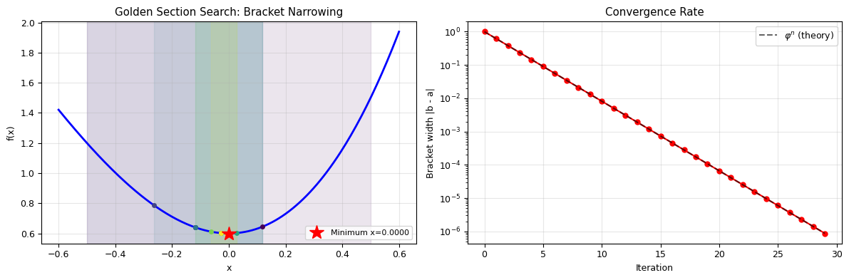
Bracket shrinks by factor φ ≈ 0.618 each step
After 29 steps: bracket width = 8.70e-07
Only 1 function evaluation per step (not 2)!
Golden Section vs Gradient Descent#
Feature |
Gradient Descent |
Golden Section |
|---|---|---|
Requires derivative? |
Yes |
No |
Requires bracket? |
No |
Yes (must contain minimum) |
Convergence |
Depends on step size |
Guaranteed linear (factor 0.618) |
Works in N-D? |
Yes |
Only 1D |
Multiple minima? |
Finds nearest |
Finds the one in the bracket |
IV. Extending to 2D: Gradient Descent on Surfaces#
2D Test Functions#
Now we extend gradient descent to functions of two variables. The gradient replaces the derivative:
where \(\mathbf{x} = (x, y)\) and \(\nabla f = \left(\frac{\partial f}{\partial x}, \frac{\partial f}{\partial y}\right)\).
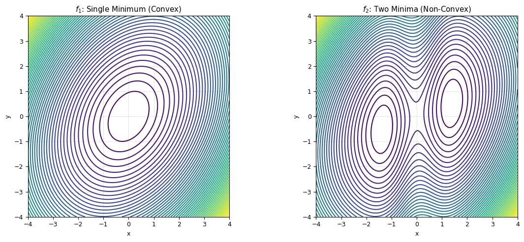
We’ll use two test functions:
\(f_1\): Single minimum (convex) $\(f_1(x, y) = \frac{x^2}{2} + \frac{y^2}{3} - \frac{xy}{4}\)$
\(f_2\): Two minima (non-convex) $\(f_2(x, y) = \frac{x^2}{2} + \frac{y^2}{3} - \frac{xy}{4} + 3 e^{-x^2}\)$
The Gaussian bump in \(f_2\) creates a second local minimum.
def f1(x):
    """Simple function with 1 minimum."""
    return x[0]**2 / 2 + x[1]**2 / 3 - x[0] * x[1] / 4

def f2(x):
    """Function with 2 minima (Gaussian bump)."""
    return x[0]**2 / 2 + x[1]**2 / 3 - x[0] * x[1] / 4 + 3 * np.exp(-x[0]**2)

# Visualize both functions
x_min, x_max = -4, 4
y_min, y_max = -4, 4
nx = np.linspace(x_min, x_max, 400)
ny = np.linspace(y_min, y_max, 400)
x, y = np.meshgrid(nx, ny)

fig, axes = plt.subplots(1, 2, figsize=(12, 5))

z1 = f1([x, y])
levels1 = np.arange(np.min(z1), np.max(z1), 0.3)
axes[0].contour(x, y, z1, levels=levels1, cmap='viridis')
axes[0].set_xlabel('x')
axes[0].set_ylabel('y')
axes[0].set_title('$f_1$: Single Minimum (Convex)')
axes[0].set_aspect('equal')
axes[0].grid(alpha=0.3)

z2 = f2([x, y])
levels2 = np.arange(np.min(z2), np.max(z2), 0.3)
axes[1].contour(x, y, z2, levels=levels2, cmap='viridis')
axes[1].set_xlabel('x')
axes[1].set_ylabel('y')
axes[1].set_title('$f_2$: Two Minima (Non-Convex)')
axes[1].set_aspect('equal')
axes[1].grid(alpha=0.3)

plt.tight_layout()
plt.show()
2D Numerical Gradient#
We compute the gradient using central differences in each direction:
def derivative2(f, xy, d=0.001):
    """Numerical gradient of a 2D function using central differences."""
    x, y = xy[0], xy[1]
    fx = (f([x + d/2, y]) - f([x - d/2, y])) / d
    fy = (f([x, y + d/2]) - f([x, y - d/2])) / d
    return np.array([fx, fy])

def init(x_min, x_max, y_min, y_max):
    """Generate random starting point in [x_min, x_max] x [y_min, y_max]."""
    x0 = x_min + np.random.random() * (x_max - x_min)
    y0 = y_min + np.random.random() * (y_max - y_min)
    return [x0, y0]

# Test the gradient
test_point = [1.0, 2.0]
grad = derivative2(f1, test_point)
print(f"Gradient of f1 at (1, 2): [{grad[0]:.4f}, {grad[1]:.4f}]")
print(f"Analytical: [{1.0 - 2.0/4:.4f}, {2*2.0/3 - 1.0/4:.4f}]")
Gradient of f1 at (1, 2): [0.5000, 1.0833]
Analytical: [0.5000, 1.0833]
Method 1: Fixed Step Size in 2D#
def minimize_fix(f, x0, dx=0.05, N=1000):
    """2D gradient descent with fixed step size."""
    x_now = np.array(x0, dtype=float)
    converged = False
    x_hist = [x_now.copy()]

    for i in range(N):
        # code...
        x_next = x_now - dx * derivative2(f, x_now)

        if np.linalg.norm(x_next - x_now) < 1e-6:
            converged = True
            break
        else:
            x_now = x_next
            x_hist.append(x_now.copy())

    return converged, np.array(x_hist), f(x_now)

# Test on f1 (single minimum)
x0, y0 = 3.5, 3.5
converged, x_hist, f_min = minimize_fix(f1, [x0, y0], dx=0.1)

z1 = f1([x, y])
plt.figure(figsize=(6, 5))
plt.contour(x, y, z1, levels=np.arange(0, np.max(z1), 0.3), cmap='viridis')
plt.plot(x_hist[:, 0], x_hist[:, 1], 'ro-', ms=3, lw=1, label='Path')
plt.plot(x0, y0, 'go', ms=10, label='Start')
plt.plot(x_hist[-1, 0], x_hist[-1, 1], 'k*', ms=15, label='Solution')
plt.xlabel('x')
plt.ylabel('y')
plt.title(f'Fixed Step on $f_1$: {len(x_hist)} iterations')
plt.legend(fontsize=8)
plt.grid(alpha=0.3)
plt.show()

print(f'Converged: {converged}')
print(f'Start: ({x0}, {y0}), f = {f1([x0, y0]):.4f}')
print(f'End:   ({x_hist[-1, 0]:.4f}, {x_hist[-1, 1]:.4f}), f = {f_min:.4f}')
print(f'Iterations: {len(x_hist)}')
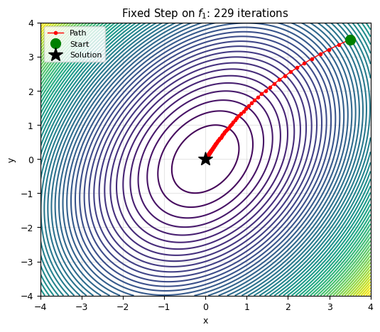
Converged: True
Start: (3.5, 3.5), f = 7.1458
End:   (0.0000, 0.0000), f = 0.0000
Iterations: 229
# Test on f2 (two minima) — starting point determines which minimum we find
fig, axes = plt.subplots(1, 2, figsize=(12, 5))

z2 = f2([x, y])
levels2 = np.arange(np.min(z2), np.max(z2), 0.3)

# Start from right side
converged, x_hist_r, f_min_r = minimize_fix(f2, [3.5, 3.5])
axes[0].contour(x, y, z2, levels=levels2, cmap='viridis')
axes[0].plot(x_hist_r[:, 0], x_hist_r[:, 1], 'ro-', ms=3, lw=1)
axes[0].plot(3.5, 3.5, 'go', ms=10)
axes[0].plot(x_hist_r[-1, 0], x_hist_r[-1, 1], 'k*', ms=15)
axes[0].set_title(f'Start (3.5, 3.5) → ({x_hist_r[-1,0]:.2f}, {x_hist_r[-1,1]:.2f})')
axes[0].set_xlabel('x')
axes[0].set_ylabel('y')
axes[0].grid(alpha=0.3)

# Start from left side
converged, x_hist_l, f_min_l = minimize_fix(f2, [-3.5, 3.5])
axes[1].contour(x, y, z2, levels=levels2, cmap='viridis')
axes[1].plot(x_hist_l[:, 0], x_hist_l[:, 1], 'ro-', ms=3, lw=1)
axes[1].plot(-3.5, 3.5, 'go', ms=10)
axes[1].plot(x_hist_l[-1, 0], x_hist_l[-1, 1], 'k*', ms=15)
axes[1].set_title(f'Start (-3.5, 3.5) → ({x_hist_l[-1,0]:.2f}, {x_hist_l[-1,1]:.2f})')
axes[1].set_xlabel('x')
axes[1].set_ylabel('y')
axes[1].grid(alpha=0.3)

plt.suptitle('Fixed Step on $f_2$: Different Starts → Different Minima', fontsize=11)
plt.tight_layout()
plt.show()

print(f"Right start → f = {f_min_r:.4f} ({len(x_hist_r)} steps)")
print(f"Left start  → f = {f_min_l:.4f} ({len(x_hist_l)} steps)")
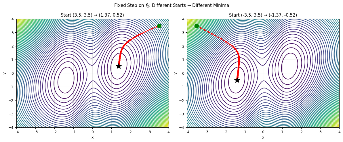
Right start → f = 1.3096 (355 steps)
Left start  → f = 1.3096 (358 steps)
Method 2: Variable Step Size (Barzilai-Borwein) in 2D#
The 2D generalization of the Barzilai-Borwein method:
def minimize_var(f, x0, N=1000):
    """2D gradient descent with Barzilai-Borwein variable step size."""
    x_now = np.array(x0, dtype=float)
    x_prev = None
    converged = False
    x_hist = [x_now.copy()]

    for i in range(N):
        df_now = derivative2(f, x_now)

        if x_prev is None:
            dx = 0.01
        else:
            df_prev = derivative2(f, x_prev)
            dd = df_now - df_prev
            denom = np.linalg.norm(dd)**2
            if denom > 1e-16:
                dx = np.dot(x_now - x_prev, dd) / denom
            else:
                dx = 0.01

        x_next = x_now - df_now * dx

        if f(x_next) < f(x_now):
            x_prev = x_now.copy()
            x_now = x_next
            x_hist.append(x_now.copy())
        else:
            converged = True
            break

    return converged, np.array(x_hist), f(x_now)
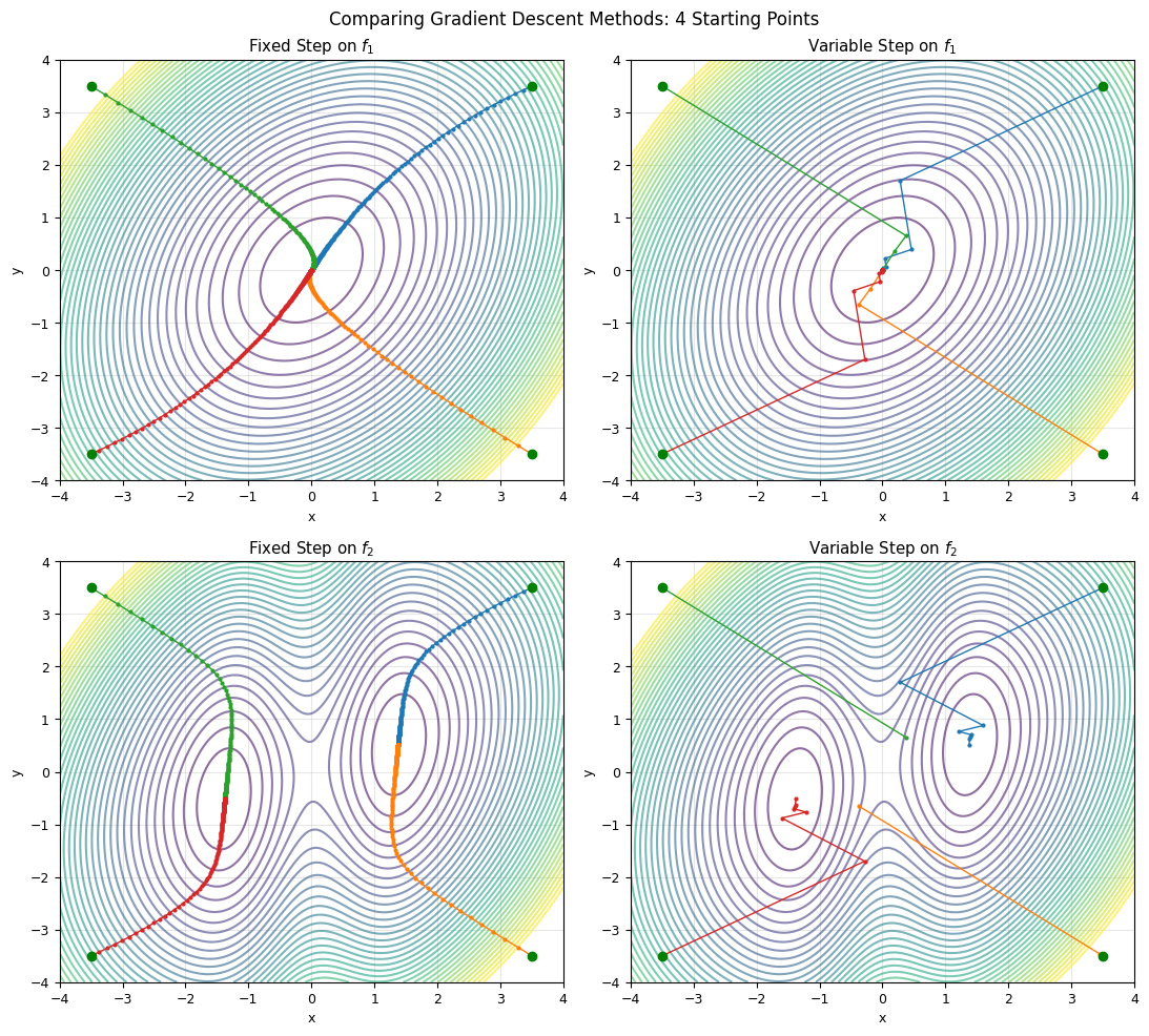
Comparing Both Methods in 2D#
# Compare both methods on f1 and f2
start_points = [[3.5, 3.5], [3.5, -3.5], [-3.5, 3.5], [-3.5, -3.5]]
methods = [
    ('Fixed Step', minimize_fix),
    ('Variable Step', minimize_var),
]

fig, axes = plt.subplots(2, 2, figsize=(11, 10))

for col, (name, method) in enumerate(methods):
    # f1 (top row)
    axes[0, col].contour(x, y, f1([x, y]),
                         levels=np.arange(0, 12, 0.3), cmap='viridis', alpha=0.6)
    for sp in start_points:
        conv, xh, fm = method(f1, sp)
        axes[0, col].plot(xh[:, 0], xh[:, 1], 'o-', ms=2, lw=1)
        axes[0, col].plot(sp[0], sp[1], 'go', ms=6)
    axes[0, col].set_title(f'{name} on $f_1$')
    axes[0, col].set_xlabel('x')
    axes[0, col].set_ylabel('y')
    axes[0, col].grid(alpha=0.3)

    # f2 (bottom row)
    axes[1, col].contour(x, y, f2([x, y]),
                         levels=np.arange(np.min(z2), 12, 0.3), cmap='viridis', alpha=0.6)
    for sp in start_points:
        conv, xh, fm = method(f2, sp)
        axes[1, col].plot(xh[:, 0], xh[:, 1], 'o-', ms=2, lw=1)
        axes[1, col].plot(sp[0], sp[1], 'go', ms=6)
    axes[1, col].set_title(f'{name} on $f_2$')
    axes[1, col].set_xlabel('x')
    axes[1, col].set_ylabel('y')
    axes[1, col].grid(alpha=0.3)

plt.suptitle('Comparing Gradient Descent Methods: 4 Starting Points', fontsize=12)
plt.tight_layout()
plt.show()
# Quantitative comparison on f2
print("Comparison on f2 (two minima)")
print(f'{"Start":>14s} | {"Method":>12s} | {"Conv":>5s} | {"Final (x, y)":>20s} | {"f_min":>8s} | {"Steps":>5s}')
print('-' * 80)

for sp in start_points:
    for name, method in methods:
        conv, xh, fm = method(f2, sp)
        end = xh[-1]
        print(f'({sp[0]:5.1f},{sp[1]:5.1f}) | {name:>12s} | {str(conv):>5s} | ({end[0]:8.4f}, {end[1]:8.4f}) | {fm:8.4f} | {len(xh):5d}')
    print()
Comparison on f2 (two minima)
         Start |       Method |  Conv |         Final (x, y) |    f_min | Steps
--------------------------------------------------------------------------------
(  3.5,  3.5) |   Fixed Step |  True | (  1.3748,   0.5156) |   1.3096 |   355
(  3.5,  3.5) | Variable Step |  True | (  1.3762,   0.5162) |   1.3096 |     9

(  3.5, -3.5) |   Fixed Step |  True | (  1.3748,   0.5155) |   1.3096 |   358
(  3.5, -3.5) | Variable Step |  True | ( -0.3739,  -0.6540) |   2.7599 |     3

( -3.5,  3.5) |   Fixed Step |  True | ( -1.3748,  -0.5155) |   1.3096 |   358
( -3.5,  3.5) | Variable Step |  True | (  0.3739,   0.6540) |   2.7599 |     3

( -3.5, -3.5) |   Fixed Step |  True | ( -1.3748,  -0.5156) |   1.3096 |   355
( -3.5, -3.5) | Variable Step |  True | ( -1.3762,  -0.5162) |   1.3096 |     9
V. Using scipy.optimize#
Professional Optimization with scipy.optimize.minimize#
In practice, we use well-tested library implementations. scipy.optimize.minimize provides many algorithms through a unified interface:
Method |
Type |
Requires |
Best for |
|---|---|---|---|
|
Simplex (gradient-free) |
Only \(f\) |
Noisy or non-smooth functions |
|
Direction set (gradient-free) |
Only \(f\) |
Low-dimensional smooth functions |
|
Conjugate gradient |
\(f\), \(\nabla f\) |
Large-scale smooth problems |
|
Quasi-Newton |
\(f\), \(\nabla f\) |
General smooth optimization |
|
Newton + CG |
\(f\), \(\nabla f\), \(H\) |
When Hessian is available |
We’ll study Newton, BFGS, and CG in detail in the next lecture. For now, let’s see them in action.
from scipy.optimize import minimize as sp_minimize

x0 = [3.5, 3.5]

print(f"Minimizing f2 from starting point {x0}")
print("=" * 60)

for method in ['Nelder-Mead', 'Powell', 'CG', 'BFGS']:
    res = sp_minimize(f2, x0, method=method, tol=1e-6)
    print(f"\n{method}:")
    print(f"  Solution: ({res.x[0]:.6f}, {res.x[1]:.6f})")
    print(f"  f_min:    {res.fun:.6f}")
    print(f"  Evaluations: {res.nfev}")
    print(f"  Converged: {res.success}")
Minimizing f2 from starting point [3.5, 3.5]
============================================================

Nelder-Mead:
  Solution: (1.374845, 0.515567)
  f_min:    1.309622
  Evaluations: 114
  Converged: True

Powell:
  Solution: (1.374845, 0.515567)
  f_min:    1.309622
  Evaluations: 126
  Converged: True

CG:
  Solution: (-1.374845, -0.515566)
  f_min:    1.309622
  Evaluations: 60
  Converged: True

BFGS:
  Solution: (1.374845, 0.515567)
  f_min:    1.309622
  Evaluations: 27
  Converged: True
# Visual comparison: our methods vs scipy
fig, axes = plt.subplots(1, 2, figsize=(12, 5))

z2 = f2([x, y])
levels2 = np.arange(np.min(z2), np.max(z2), 0.3)

# Left: our variable step method
conv, xh_ours, fm = minimize_var(f2, [3.5, -3.5])
axes[0].contour(x, y, z2, levels=levels2, cmap='viridis', alpha=0.6)
axes[0].plot(xh_ours[:, 0], xh_ours[:, 1], 'ro-', ms=3, lw=1)
axes[0].set_title(f'Our Variable Step ({len(xh_ours)} steps)')
axes[0].set_xlabel('x')
axes[0].set_ylabel('y')
axes[0].grid(alpha=0.3)

# Right: scipy BFGS (collect trajectory using callback)
trajectory = [[3.5, -3.5]]
def callback(xk):
    trajectory.append(xk.tolist())

res = sp_minimize(f2, [3.5, 3.5], method='BFGS', callback=callback, tol=1e-6)
traj = np.array(trajectory)

axes[1].contour(x, y, z2, levels=levels2, cmap='viridis', alpha=0.6)
axes[1].plot(traj[:, 0], traj[:, 1], 'ro-', ms=3, lw=1)
axes[1].set_title(f'scipy BFGS ({len(traj)} steps)')
axes[1].set_xlabel('x')
axes[1].set_ylabel('y')
axes[1].grid(alpha=0.3)

plt.suptitle('Our Method vs scipy on $f_2$', fontsize=11)
plt.tight_layout()
plt.show()

print(f"Our method: {len(xh_ours)} steps, f = {fm:.6f}")
print(f"scipy BFGS: {len(traj)} steps, f = {res.fun:.6f}")
print(f"\nBFGS is much more efficient — we'll learn why in the next lecture!")
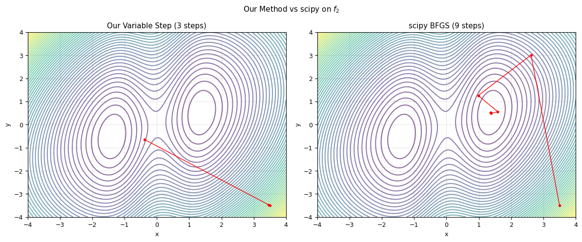
Our method: 3 steps, f = 2.759868
scipy BFGS: 9 steps, f = 1.309622

BFGS is much more efficient — we'll learn why in the next lecture!
Summary: What We Learned Today#
Method |
Derivatives? |
Dimension |
Key Idea |
|---|---|---|---|
Gradient descent (fixed \(\eta\)) |
Yes |
Any |
Simple but sensitive to \(\eta\) |
Barzilai-Borwein (variable \(\eta\)) |
Yes |
Any |
Adapts \(\eta\) from previous step |
Golden section search |
No |
1D only |
Bracket narrowing via golden ratio |
Nelder-Mead (scipy) |
No |
Any |
Simplex exploration |
BFGS (scipy) |
Yes |
Any |
Quasi-Newton (next lecture!) |