Lecture 16: Optimization II — Newton’s Method, BFGS, and Conjugate Gradient#
Beyond Gradient Descent: Using Curvature#
In Lecture 15, we built gradient descent optimizers — they only use the first derivative (gradient) to decide which direction to step.
The key limitation: gradient descent doesn’t know the shape of the landscape. Is the valley wide and flat, or narrow and steep? A method that uses curvature (second derivative) can adapt its step to the local geometry.
import numpy as np
import matplotlib.pyplot as plt
from scipy.optimize import minimize as sp_minimize
I. Newton’s Method: Quadratic Convergence#
The Idea: Fit a Quadratic, Jump to Its Minimum#
Gradient descent uses a linear approximation of \(f\) at the current point. Newton’s method uses a quadratic approximation (Taylor expansion to second order):
where \(\mathbf{H}\) is the Hessian matrix of second partial derivatives:
Setting the gradient of the quadratic model to zero gives the Newton step:
For a quadratic function, Newton’s method converges in one step — it jumps directly to the minimum!
For general functions, convergence is quadratic: the error squares at each step (\(\epsilon_{n+1} \propto \epsilon_n^2\)). Compare this to gradient descent’s linear convergence (\(\epsilon_{n+1} \propto c \cdot \epsilon_n\)).
1D Newton’s Method: Root Finding Meets Optimization#
In 1D, the Hessian is just \(f''(x)\), and the Newton step becomes:
This is equivalent to finding the root of the derivative — exactly Newton-Raphson applied to \(f'(x) = 0\).
# Reuse our test function from Lecture 15
A, B, C = 1.2, 3.0, 0.6

def f(x):
    return A * x**3 + B * x**2 + C

def f_prime(x):
    return 3 * A * x**2 + 2 * B * x

def f_double_prime(x):
    return 6 * A * x + 2 * B

# 1D Newton's method
def newton_1d(x0, N=50, tol=1e-10):
    x = x0
    x_hist = [x]
    for i in range(N):
        ## code ...
        fp = f_prime(x)
        fpp = f_double_prime(x)
        if abs(fpp) < 1e-12:
            break
        dx = -fp/fpp
        x += dx
        x_hist.append(x)
        if abs(dx) < tol:
            break

    return np.array(x_hist)

# Compare: gradient descent vs Newton
def gradient_descent_1d(x0, eta=0.01, N=200, tol=1e-10):
    x = x0
    x_hist = [x]
    for i in range(N):
        dx = -eta * f_prime(x)
        x = x + dx
        x_hist.append(x)
        if abs(dx) < tol:
            break
    return np.array(x_hist)

x0 = 2.0
xh_gd = gradient_descent_1d(x0, eta=0.01)
xh_newton = newton_1d(x0)

fig, axes = plt.subplots(1, 2, figsize=(12, 4))

# Left: trajectories
xp = np.linspace(-3, 3, 300)
axes[0].plot(xp, f(xp), 'k-', lw=2)
axes[0].plot(xh_gd, f(xh_gd), 'bo-', ms=4, label=f'GD ({len(xh_gd)} steps)')
axes[0].plot(xh_newton, f(xh_newton), 'rs-', ms=6, label=f'Newton ({len(xh_newton)} steps)')
axes[0].set_xlabel('x')
axes[0].set_ylabel('f(x)')
axes[0].set_title('Gradient Descent vs Newton')
axes[0].legend()
axes[0].grid(alpha=0.3)

# Right: convergence
axes[1].semilogy(range(len(xh_gd)), np.abs(f_prime(xh_gd)), 'bo-', ms=3, label='Gradient Descent')
axes[1].semilogy(range(len(xh_newton)), np.abs(f_prime(xh_newton)), 'rs-', ms=5, label="Newton's Method")
axes[1].set_xlabel('Iteration')
axes[1].set_ylabel("|f'(x)|")
axes[1].set_title('Convergence Rate')
axes[1].legend()
axes[1].grid(alpha=0.3)

plt.tight_layout()
plt.show()

print(f'Gradient descent: {len(xh_gd)-1} steps, x* = {xh_gd[-1]:.8f}')
print(f"Newton's method:  {len(xh_newton)-1} steps, x* = {xh_newton[-1]:.8f}")
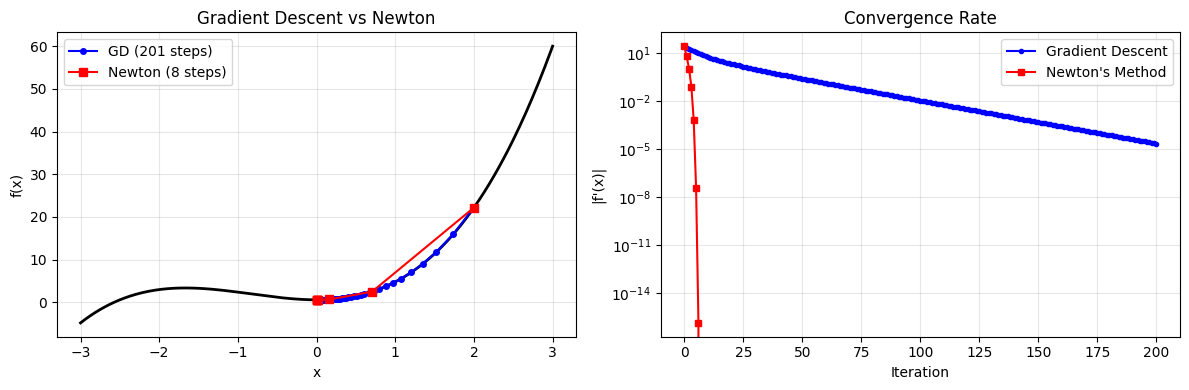
Gradient descent: 200 steps, x* = 0.00000365
Newton's method:  7 steps, x* = 0.00000000
Extending to 2D: The Hessian Matrix#
For a function \(f(x, y)\), the Hessian is:
We compute it numerically using central differences.
# Test functions from Lecture 15
def f1(x):
    return x[0]**2 / 2 + x[1]**2 / 3 - x[0] * x[1] / 4

def f2(x):
    return x[0]**2 / 2 + x[1]**2 / 3 - x[0] * x[1] / 4 + 3 * np.exp(-x[0]**2)

# Numerical gradient (central difference)
def derivative2(f, xy, d=0.001):
    x, y = xy[0], xy[1]
    fx = (f([x + d/2, y]) - f([x - d/2, y])) / d
    fy = (f([x, y + d/2]) - f([x, y - d/2])) / d
    return np.array([fx, fy])

# Numerical Hessian (central difference)
def hessian2(f, xy, d=0.001):
    x, y = xy[0], xy[1]
    fxx = (f([x+d, y]) - 2*f([x, y]) + f([x-d, y])) / d**2
    fyy = (f([x, y+d]) - 2*f([x, y]) + f([x, y-d])) / d**2
    fxy = (f([x+d/2, y+d/2]) - f([x+d/2, y-d/2])
         - f([x-d/2, y+d/2]) + f([x-d/2, y-d/2])) / d**2
    return np.array([[fxx, fxy],
                     [fxy, fyy]])

# Grid for contour plots
x_min, x_max = -4, 4
nx = np.linspace(x_min, x_max, 400)
x, y = np.meshgrid(nx, nx)
def minimize_newton(f, x0, N=100, tol=1e-8):
    """2D Newton's method using numerical Hessian."""
    x_now = np.array(x0, dtype=float)
    x_hist = [x_now.copy()]

    for i in range(N):
        grad = derivative2(f, x_now)
        H = hessian2(f, x_now)

        # Newton step: dx = -H^{-1} grad
        try:
            dx = np.linalg.solve(H, -grad)
        except np.linalg.LinAlgError:
            break  # Singular Hessian

        x_next = x_now + dx
        x_hist.append(x_next.copy())

        if np.linalg.norm(dx) < tol:
            break

        x_now = x_next

    return True, np.array(x_hist), f(x_now)
# Newton on f1 (nearly quadratic) -- expect very fast convergence
conv, xh_n, fm = minimize_newton(f1, [3.5, 3.5])

z1 = f1([x, y])
levels1 = np.arange(0, 12, 0.3)

fig, ax = plt.subplots(figsize=(6, 5))
ax.contour(x, y, z1, levels=levels1, cmap='viridis', alpha=0.6)
ax.plot(xh_n[:, 0], xh_n[:, 1], 'ro-', ms=6, lw=2)
ax.plot(xh_n[0, 0], xh_n[0, 1], 'go', ms=10, label='Start')
ax.plot(xh_n[-1, 0], xh_n[-1, 1], 'r*', ms=15, label='End')
ax.set_title(f"Newton's method on f1: {len(xh_n)-1} steps!")
ax.set_xlabel('x')
ax.set_ylabel('y')
ax.legend()
ax.grid(alpha=0.3)
plt.tight_layout()
plt.show()

print(f'Steps: {len(xh_n)-1}')
print(f'Minimum at: ({xh_n[-1,0]:.8f}, {xh_n[-1,1]:.8f})')
print(f'f_min = {fm:.10f}')
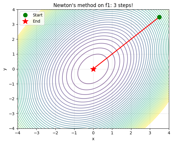
Steps: 3
Minimum at: (0.00000000, 0.00000000)
f_min = 0.0000000000
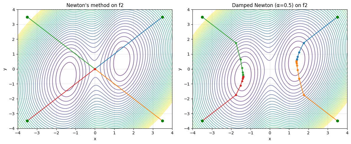
When Newton’s Method Fails#
Newton’s method is powerful but has important limitations:
Non-convex functions: If the Hessian has negative eigenvalues, the Newton step may go to a maximum or saddle point instead of a minimum
Far from minimum: The quadratic approximation may be poor, causing the step to overshoot wildly
Singular Hessian: At inflection points, \(\det(\mathbf{H}) = 0\) and the method breaks down
A practical fix: damped Newton — take only a fraction of the Newton step: $\(\mathbf{x}_{n+1} = \mathbf{x}_n + \alpha \, \Delta\mathbf{x}_\text{Newton}, \quad 0 < \alpha \leq 1\)$
# Newton on f2 from different starting points
start_points = [[3.5, 3.5], [3.5, -3.5], [-3.5, 3.5], [-3.5, -3.5]]

z2 = f2([x, y])
levels2 = np.arange(np.min(z2), 12, 0.3)

fig, axes = plt.subplots(1, 2, figsize=(12, 5))

# Newton
axes[0].contour(x, y, z2, levels=levels2, cmap='viridis', alpha=0.6)
for sp in start_points:
    conv, xh, fm = minimize_newton(f2, sp)
    axes[0].plot(xh[:, 0], xh[:, 1], 'o-', ms=4, lw=1.5)
    axes[0].plot(sp[0], sp[1], 'go', ms=6)
axes[0].set_title("Newton's method on f2")
axes[0].set_xlabel('x')
axes[0].set_ylabel('y')
axes[0].grid(alpha=0.3)

# Damped Newton
def minimize_damped_newton(f, x0, alpha=0.5, N=200, tol=1e-8):
    x_now = np.array(x0, dtype=float)
    x_hist = [x_now.copy()]
    for i in range(N):
        grad = derivative2(f, x_now)
        H = hessian2(f, x_now)
        try:
            dx = np.linalg.solve(H, -grad)
        except np.linalg.LinAlgError:
            break
        x_next = x_now + alpha * dx
        x_hist.append(x_next.copy())
        if np.linalg.norm(alpha * dx) < tol:
            break
        x_now = x_next
    return True, np.array(x_hist), f(x_now)

axes[1].contour(x, y, z2, levels=levels2, cmap='viridis', alpha=0.6)
for sp in start_points:
    conv, xh, fm = minimize_damped_newton(f2, sp, alpha=0.5)
    axes[1].plot(xh[:, 0], xh[:, 1], 'o-', ms=4, lw=1.5)
    axes[1].plot(sp[0], sp[1], 'go', ms=6)
axes[1].set_title("Damped Newton (\u03b1=0.5) on f2")
axes[1].set_xlabel('x')
axes[1].set_ylabel('y')
axes[1].grid(alpha=0.3)

plt.tight_layout()
plt.show()
Cost Analysis#
Gradient Descent |
Newton’s Method |
|
|---|---|---|
Per step |
1 gradient evaluation (\(n\) function calls) |
1 gradient + 1 Hessian (\(n + n^2\) calls) + solve \(n \times n\) system |
Convergence |
Linear: \(\epsilon_{n+1} \approx c \cdot \epsilon_n\) |
Quadratic: \(\epsilon_{n+1} \approx C \cdot \epsilon_n^2\) |
Total steps |
Many (100s–1000s) |
Few (5–20) |
Scaling |
\(O(n)\) per step |
\(O(n^3)\) per step (matrix solve) |
For small problems (\(n \lesssim 100\)), Newton’s method wins easily.
For large problems (\(n \gg 1000\)), the \(O(n^3)\) cost per step becomes prohibitive.
Can we get Newton-like convergence without computing the full Hessian? → Yes! That’s the idea behind BFGS and conjugate gradient.
II. Conjugate Gradient: Smart Search Directions#
The Problem with Gradient Descent#
Look at the path gradient descent takes on an elliptical valley — it zigzags! Each step is perpendicular to the previous one (the new gradient is orthogonal to the old step), so it keeps revisiting the same directions.
Conjugate gradient (CG) fixes this by choosing search directions that are conjugate (or \(\mathbf{H}\)-orthogonal):
This ensures each direction explores a new dimension of the landscape. For a quadratic function in \(n\) dimensions, CG converges in exactly \(n\) steps!
The Algorithm (Fletcher-Reeves)#
Start: \(\mathbf{d}_0 = -\nabla f(\mathbf{x}_0)\) (steepest descent direction)
Line search: find \(\alpha_k\) that minimizes \(f(\mathbf{x}_k + \alpha_k \mathbf{d}_k)\)
Update: \(\mathbf{x}_{k+1} = \mathbf{x}_k + \alpha_k \mathbf{d}_k\)
New direction: \(\mathbf{d}_{k+1} = -\nabla f(\mathbf{x}_{k+1}) + \beta_k \mathbf{d}_k\)
where \(\beta_k = \frac{\|\nabla f(\mathbf{x}_{k+1})\|^2}{\|\nabla f(\mathbf{x}_k)\|^2}\) (Fletcher-Reeves formula)
The \(\beta_k\) term adds a fraction of the previous direction — this prevents the zigzagging.
def line_search_golden(f_1d, a=-1, b=1, tol=1e-6):
    """1D golden section search for line search."""
    phi = (np.sqrt(5) - 1) / 2
    x1 = b - phi * (b - a)
    x2 = a + phi * (b - a)
    f1, f2_val = f_1d(x1), f_1d(x2)
    for _ in range(100):
        if (b - a) < tol:
            break
        if f1 < f2_val:
            b = x2
            x2, f2_val = x1, f1
            x1 = b - phi * (b - a)
            f1 = f_1d(x1)
        else:
            a = x1
            x1, f1 = x2, f2_val
            x2 = a + phi * (b - a)
            f2_val = f_1d(x2)
    return (a + b) / 2

def minimize_cg(f, x0, N=200, tol=1e-8):
    """Conjugate gradient with Fletcher-Reeves formula."""
    x_now = np.array(x0, dtype=float)
    grad = derivative2(f, x_now)
    d = -grad.copy()  # Initial direction = steepest descent
    x_hist = [x_now.copy()]

    for k in range(N):
        # Line search along direction d
        f_1d = lambda alpha, xn=x_now, dn=d: f(xn + alpha * dn)
        alpha = line_search_golden(f_1d, a=0, b=2.0)

        x_next = x_now + alpha * d
        x_hist.append(x_next.copy())

        if np.linalg.norm(x_next - x_now) < tol:
            break

        ## code .....
        grad_new = derivative2(f, x_next)
        # fprime= np.dot(grad,grad)
        # if  fprime < 1e-12:  fprime = 1e-12

        beta = np.dot(grad_new, grad_new) / max(np.dot(grad, grad), 1e-12)
        d = -grad_new + beta * d
        grad = grad_new
        x_now = x_next

    return True, np.array(x_hist), f(x_now)
# Compare gradient descent vs conjugate gradient on f1
def minimize_fix(f, x0, dx=0.05, N=1000):
    x_now = np.array(x0, dtype=float)
    x_hist = [x_now.copy()]
    for i in range(N):
        dfx = derivative2(f, x_now)
        x_next = x_now - dx * dfx
        if np.linalg.norm(x_next - x_now) < 1e-6:
            break
        x_now = x_next
        x_hist.append(x_now.copy())
    return True, np.array(x_hist), f(x_now)

sp = [3.5, 3.5]
_, xh_gd, _ = minimize_fix(f1, sp)
_, xh_cg, _ = minimize_cg(f1, sp)

z1 = f1([x, y])
fig, axes = plt.subplots(1, 2, figsize=(12, 5))

axes[0].contour(x, y, z1, levels=np.arange(0, 12, 0.3), cmap='viridis', alpha=0.6)
axes[0].plot(xh_gd[:, 0], xh_gd[:, 1], 'ro-', ms=2, lw=1)
axes[0].plot(sp[0], sp[1], 'go', ms=8)
axes[0].set_title(f'Gradient Descent: {len(xh_gd)-1} steps')
axes[0].set_xlabel('x')
axes[0].set_ylabel('y')
axes[0].grid(alpha=0.3)

axes[1].contour(x, y, z1, levels=np.arange(0, 12, 0.3), cmap='viridis', alpha=0.6)
axes[1].plot(xh_cg[:, 0], xh_cg[:, 1], 'ro-', ms=4, lw=1.5)
axes[1].plot(sp[0], sp[1], 'go', ms=8)
axes[1].set_title(f'Conjugate Gradient: {len(xh_cg)-1} steps')
axes[1].set_xlabel('x')
axes[1].set_ylabel('y')
axes[1].grid(alpha=0.3)

plt.suptitle('Zigzagging (GD) vs Straight Path (CG) on f1', fontsize=12)
plt.tight_layout()
plt.show()

print(f'Gradient descent: {len(xh_gd)-1} steps')
print(f'Conjugate gradient: {len(xh_cg)-1} steps')
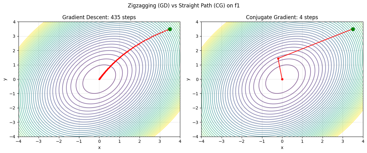
Gradient descent: 435 steps
Conjugate gradient: 4 steps
III. BFGS: The Best of Both Worlds#
Quasi-Newton Methods: Approximate the Hessian#
Newton’s method needs the exact Hessian (\(O(n^2)\) second derivatives). Quasi-Newton methods build an approximation to the Hessian (or its inverse) using only gradient information — updating it step by step.
BFGS (Broyden–Fletcher–Goldfarb–Shanno) is the most successful quasi-Newton method:
Start with \(\mathbf{B}_0 = \mathbf{I}\) (identity matrix — pretend the Hessian is the identity)
Compute search direction: \(\mathbf{d}_k = -\mathbf{B}_k^{-1} \nabla f(\mathbf{x}_k)\)
Line search: find step size \(\alpha_k\)
Update position: \(\mathbf{x}_{k+1} = \mathbf{x}_k + \alpha_k \mathbf{d}_k\)
Update the Hessian approximation using the secant condition:
where \(\mathbf{s}_k = \mathbf{x}_{k+1} - \mathbf{x}_k\) and \(\mathbf{y}_k = \nabla f(\mathbf{x}_{k+1}) - \nabla f(\mathbf{x}_k)\).
Key insight: BFGS “learns” the curvature from how the gradient changes — no second derivatives needed!
def minimize_bfgs(f, x0, N=200, tol=1e-8):
    """BFGS quasi-Newton method."""
    n = len(x0)
    x_now = np.array(x0, dtype=float)
    B = np.eye(n)  # Initial Hessian approximation = identity
    grad = derivative2(f, x_now)
    x_hist = [x_now.copy()]

    for k in range(N):
        # Search direction
        d = np.linalg.solve(B, -grad)

        # Line search along d
        f_1d = lambda alpha, xn=x_now, dn=d: f(xn + alpha * dn)
        alpha = line_search_golden(f_1d, a=0, b=2.0)

        s = alpha * d  # Step
        x_next = x_now + s
        x_hist.append(x_next.copy())

        if np.linalg.norm(s) < tol:
            break

        grad_new = derivative2(f, x_next)
        y = grad_new - grad  # Gradient change

        # BFGS update
        sy = np.dot(s, y)
        if abs(sy) > 1e-15:  # Skip update if s and y are nearly orthogonal
            Bs = B @ s
            B = B + np.outer(y, y) / sy - np.outer(Bs, Bs) / np.dot(s, Bs)

        x_now = x_next
        grad = grad_new

    return True, np.array(x_hist), f(x_now)
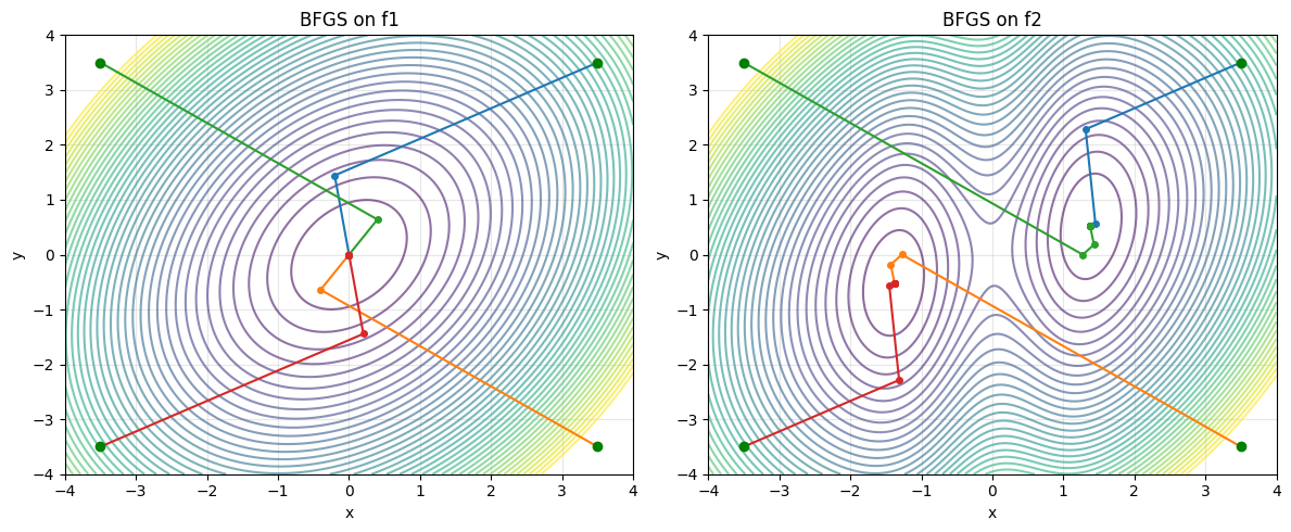
# BFGS on f1 and f2
fig, axes = plt.subplots(1, 2, figsize=(12, 5))

z1 = f1([x, y])
axes[0].contour(x, y, z1, levels=np.arange(0, 12, 0.3), cmap='viridis', alpha=0.6)
for sp in [[3.5, 3.5], [3.5, -3.5], [-3.5, 3.5], [-3.5, -3.5]]:
    conv, xh, fm = minimize_bfgs(f1, sp)
    axes[0].plot(xh[:, 0], xh[:, 1], 'o-', ms=4, lw=1.5)
    axes[0].plot(sp[0], sp[1], 'go', ms=6)
axes[0].set_title('BFGS on f1')
axes[0].set_xlabel('x')
axes[0].set_ylabel('y')
axes[0].grid(alpha=0.3)

z2 = f2([x, y])
levels2 = np.arange(np.min(z2), 12, 0.3)
axes[1].contour(x, y, z2, levels=levels2, cmap='viridis', alpha=0.6)
for sp in [[3.5, 3.5], [3.5, -3.5], [-3.5, 3.5], [-3.5, -3.5]]:
    conv, xh, fm = minimize_bfgs(f2, sp)
    axes[1].plot(xh[:, 0], xh[:, 1], 'o-', ms=4, lw=1.5)
    axes[1].plot(sp[0], sp[1], 'go', ms=6)
axes[1].set_title('BFGS on f2')
axes[1].set_xlabel('x')
axes[1].set_ylabel('y')
axes[1].grid(alpha=0.3)

plt.tight_layout()
plt.show()
IV. Method Showdown: Comparing All Approaches#
# Variable step (Barzilai-Borwein) from Lecture 15
def minimize_var(f, x0, N=1000):
    x_now = np.array(x0, dtype=float)
    x_prev = None
    converged = False
    x_hist = [x_now.copy()]
    for i in range(N):
        df_now = derivative2(f, x_now)
        if x_prev is None:
            dx = 0.01
        else:
            df_prev = derivative2(f, x_prev)
            dd = df_now - df_prev
            dx = np.dot((x_now - x_prev), dd) / (np.linalg.norm(dd))**2
        x_next = x_now - df_now * dx
        if f(x_next) < f(x_now):
            x_prev = x_now
            x_now = x_next
            x_hist.append(x_now.copy())
        else:
            converged = True
            break
    return converged, np.array(x_hist), f(x_now)
# Grand comparison: all methods on f2
start_points = [[3.5, 3.5], [3.5, -3.5], [-3.5, 3.5], [-3.5, -3.5]]
methods = [
    ('Fixed Step', minimize_fix),
    ('Barzilai-Borwein', minimize_var),
    ('Newton', minimize_newton),
    ('Conjugate Grad', minimize_cg),
    ('BFGS', minimize_bfgs),
]

fig, axes = plt.subplots(2, 3, figsize=(16, 10))
axes_flat = axes.flatten()

z2 = f2([x, y])
levels2 = np.arange(np.min(z2), 12, 0.3)

for col, (name, method) in enumerate(methods):
    ax = axes_flat[col]
    ax.contour(x, y, z2, levels=levels2, cmap='viridis', alpha=0.6)
    for sp in start_points:
        conv, xh, fm = method(f2, sp)
        ax.plot(xh[:, 0], xh[:, 1], 'o-', ms=2, lw=1)
        ax.plot(sp[0], sp[1], 'go', ms=5)
    ax.set_title(name)
    ax.set_xlabel('x')
    ax.set_ylabel('y')
    ax.grid(alpha=0.3)

# scipy BFGS in last panel
axes_flat[5].contour(x, y, z2, levels=levels2, cmap='viridis', alpha=0.6)
for sp in start_points:
    traj = [sp]
    sp_minimize(f2, sp, method='BFGS', callback=lambda xk, sp=sp: traj.append(xk.tolist()), tol=1e-6)
    traj = np.array(traj)
    axes_flat[5].plot(traj[:, 0], traj[:, 1], 'o-', ms=2, lw=1)
    axes_flat[5].plot(sp[0], sp[1], 'go', ms=5)
axes_flat[5].set_title('scipy BFGS')
axes_flat[5].set_xlabel('x')
axes_flat[5].set_ylabel('y')
axes_flat[5].grid(alpha=0.3)

plt.suptitle('All Methods on f2 (4 Starting Points)', fontsize=13)
plt.tight_layout()
plt.show()
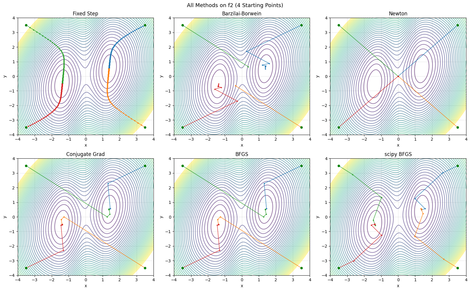
# Quantitative comparison
print('Method Comparison on f2 (two minima)')
print(f'{"Start":>14s} | {"Method":>16s} | {"Steps":>5s} | {"f_min":>8s} | {"Final (x, y)":>20s}')
print('-' * 76)

for sp in start_points:
    for name, method in methods:
        conv, xh, fm = method(f2, sp)
        end = xh[-1]
        print(f'({sp[0]:5.1f},{sp[1]:5.1f}) | {name:>16s} | {len(xh)-1:5d} | {fm:8.4f} | ({end[0]:8.4f}, {end[1]:8.4f})')
    # Also scipy BFGS
    res = sp_minimize(f2, sp, method='BFGS', tol=1e-6)
    print(f'({sp[0]:5.1f},{sp[1]:5.1f}) | {"scipy BFGS":>16s} | {res.nit:5d} | {res.fun:8.4f} | ({res.x[0]:8.4f}, {res.x[1]:8.4f})')
    print()
Method Comparison on f2 (two minima)
         Start |           Method | Steps |    f_min |         Final (x, y)
----------------------------------------------------------------------------
(  3.5,  3.5) |       Fixed Step |   354 |   1.3096 | (  1.3748,   0.5156)
(  3.5,  3.5) | Barzilai-Borwein |     8 |   1.3096 | (  1.3762,   0.5162)
(  3.5,  3.5) |           Newton |     4 |   3.0000 | (  0.0000,   0.0000)
(  3.5,  3.5) |   Conjugate Grad |    13 |   1.3096 | (  1.3748,   0.5156)
(  3.5,  3.5) |             BFGS |     6 |   1.3096 | (  1.3748,   0.5156)
(  3.5,  3.5) |       scipy BFGS |     8 |   1.3096 | (  1.3748,   0.5156)

(  3.5, -3.5) |       Fixed Step |   357 |   1.3096 | (  1.3748,   0.5155)
(  3.5, -3.5) | Barzilai-Borwein |     2 |   2.7599 | ( -0.3739,  -0.6540)
(  3.5, -3.5) |           Newton |     4 |   3.0000 | (  0.0000,  -0.0000)
(  3.5, -3.5) |   Conjugate Grad |    17 |   1.3096 | ( -1.3748,  -0.5156)
(  3.5, -3.5) |             BFGS |     7 |   1.3096 | ( -1.3748,  -0.5156)
(  3.5, -3.5) |       scipy BFGS |     7 |   1.3096 | (  1.3748,   0.5156)

( -3.5,  3.5) |       Fixed Step |   357 |   1.3096 | ( -1.3748,  -0.5155)
( -3.5,  3.5) | Barzilai-Borwein |     2 |   2.7599 | (  0.3739,   0.6540)
( -3.5,  3.5) |           Newton |     4 |   3.0000 | ( -0.0000,   0.0000)
( -3.5,  3.5) |   Conjugate Grad |    17 |   1.3096 | (  1.3748,   0.5156)
( -3.5,  3.5) |             BFGS |     7 |   1.3096 | (  1.3748,   0.5156)
( -3.5,  3.5) |       scipy BFGS |     7 |   1.3096 | ( -1.3748,  -0.5156)

( -3.5, -3.5) |       Fixed Step |   354 |   1.3096 | ( -1.3748,  -0.5156)
( -3.5, -3.5) | Barzilai-Borwein |     8 |   1.3096 | ( -1.3762,  -0.5162)
( -3.5, -3.5) |           Newton |     4 |   3.0000 | ( -0.0000,  -0.0000)
( -3.5, -3.5) |   Conjugate Grad |    13 |   1.3096 | ( -1.3748,  -0.5156)
( -3.5, -3.5) |             BFGS |     6 |   1.3096 | ( -1.3748,  -0.5156)
( -3.5, -3.5) |       scipy BFGS |     8 |   1.3096 | ( -1.3748,  -0.5156)
V. Constrained Optimization#
Optimization with Constraints#
Many physics problems have constraints:
Find the shape of a hanging chain (minimize potential energy, subject to fixed length)
Find the ground state energy (minimize \(\langle H \rangle\), subject to \(\langle\psi|\psi\rangle = 1\))
Find the equilibrium configuration (minimize free energy, subject to fixed particle number)
Mathematically: minimize \(f(\mathbf{x})\) subject to \(g(\mathbf{x}) = 0\)
Lagrange Multipliers#
The classical approach: at a constrained minimum, the gradient of \(f\) must be parallel to the gradient of \(g\):
This gives us the Lagrangian: \(\mathcal{L}(\mathbf{x}, \lambda) = f(\mathbf{x}) - \lambda \, g(\mathbf{x})\)
Setting \(\nabla_{\mathbf{x}} \mathcal{L} = 0\) and \(\partial \mathcal{L}/\partial \lambda = 0\) gives a system of equations.
Penalty Method#
A simpler computational approach: convert the constrained problem to an unconstrained one by adding a penalty for violating the constraint:
As \(\mu \to \infty\), the minimum of \(\tilde{f}\) approaches the constrained minimum of \(f\).
# Example: minimize f(x,y) = x + y  subject to  x^2 + y^2 = 1
# Find the point on the unit circle closest to the direction (-1,-1)
# Analytical answer: x* = y* = -1/sqrt(2)

def f_obj(xy):
    return xy[0] + xy[1]

def g_constraint(xy):
    return xy[0]**2 + xy[1]**2 - 1

# Penalty method: minimize f + mu * g^2
fig, axes = plt.subplots(1, 3, figsize=(15, 4))

penalties = [1, 10, 100]
theta = np.linspace(0, 2*np.pi, 200)

for idx, mu in enumerate(penalties):
    def f_penalty(xy, mu=mu):
        return f_obj(xy) + mu * g_constraint(xy)**2

    conv, xh, fm = minimize_bfgs(f_penalty, [0.5, 0.8])

    xg = np.linspace(-2, 2, 200)
    xg, yg = np.meshgrid(xg, xg)
    zp = f_obj([xg, yg]) + mu * (xg**2 + yg**2 - 1)**2
    axes[idx].contour(xg, yg, zp, levels=30, cmap='viridis', alpha=0.6)
    axes[idx].plot(np.cos(theta), np.sin(theta), 'k-', lw=2, label='Constraint')
    axes[idx].plot(xh[:, 0], xh[:, 1], 'ro-', ms=3, lw=1)
    axes[idx].plot(xh[-1, 0], xh[-1, 1], 'r*', ms=12)
    axes[idx].set_title(f'\u03bc = {mu}\n({xh[-1,0]:.3f}, {xh[-1,1]:.3f})')
    axes[idx].set_xlim(-2, 2)
    axes[idx].set_ylim(-2, 2)
    axes[idx].set_aspect('equal')
    axes[idx].grid(alpha=0.3)

plt.suptitle('Penalty Method: min(x+y) on unit circle', fontsize=12)
plt.tight_layout()
plt.show()

x_exact = -1/np.sqrt(2)
print(f'Exact solution: ({x_exact:.6f}, {x_exact:.6f})')
print(f'As mu increases, the penalty solution approaches the exact answer.')
Exact solution: (-0.707107, -0.707107)
As mu increases, the penalty solution approaches the exact answer.
# scipy with explicit constraint
constraint = {'type': 'eq', 'fun': g_constraint}

res = sp_minimize(f_obj, [0.5, 0.8], method='SLSQP', constraints=constraint)
print('scipy SLSQP (constrained optimization):')
print(f'  Solution: ({res.x[0]:.8f}, {res.x[1]:.8f})')
print(f'  f_min = {res.fun:.8f}')
print(f'  Constraint satisfied: g = {g_constraint(res.x):.2e}')
print(f'  Exact: ({-1/np.sqrt(2):.8f}, {-1/np.sqrt(2):.8f})')
scipy SLSQP (constrained optimization):
  Solution: (-0.70710678, -0.70710678)
  f_min = -1.41421356
  Constraint satisfied: g = 5.06e-10
  Exact: (-0.70710678, -0.70710678)
VI. Summary#
Method Comparison#
Method |
Convergence |
Cost per step |
Needs |
Best for |
|---|---|---|---|---|
Gradient descent |
Linear |
\(O(n)\) |
Gradient |
Simple problems, large \(n\) |
Conjugate gradient |
Superlinear |
\(O(n)\) |
Gradient + line search |
Medium \(n\), quadratic-ish |
Newton |
Quadratic |
\(O(n^3)\) |
Gradient + Hessian |
Small \(n\), exact Hessian available |
BFGS |
Superlinear |
\(O(n^2)\) |
Gradient only |
General purpose, moderate \(n\) |
Key Takeaways#
Curvature information dramatically accelerates convergence — Newton converges quadratically vs gradient descent’s linear convergence
BFGS is the practical workhorse — it approximates curvature from gradient changes, no Hessian needed
Conjugate gradient avoids zigzagging by choosing \(\mathbf{H}\)-orthogonal search directions
Constrained optimization can use penalty methods (simple) or dedicated algorithms (SLSQP, trust-constr)
All local methods find the nearest minimum — for global optimization, combine with simulated annealing (Lecture 14)
When to Use What (Practical Guide)#
Small problem (n < 100):     scipy BFGS or Newton-CG
Medium problem (n ~ 1000):   scipy L-BFGS-B (memory-limited BFGS)
Large problem (n > 10000):   scipy CG or custom gradient descent
No derivatives available:    scipy Nelder-Mead or Powell
With constraints:            scipy SLSQP or trust-constr