Lecture 17: Global Optimization I — Simulated Annealing & Basin Hopping#
PHYS 611 (Computational Physics) | Rutgers-Newark
Roadmap for L17–L19#
L17 (this lecture): Simulated Annealing, Basin Hopping, LJ clusters
L18: Evolutionary Algorithms (Genetic Algorithms, Differential Evolution)
L19: Particle Swarm Optimization, hybrid methods
By the end of L17, you will:
Understand why local optimization fails for multi-modal problems
Implement Simulated Annealing with cooling schedules
Understand Basin Hopping and when to use it
Apply these to finding global minima of Lennard-Jones clusters
import numpy as np
import matplotlib.pyplot as plt
from scipy.optimize import minimize, basinhopping
from mpl_toolkits.mplot3d import Axes3D

# Set random seed for reproducibility
np.random.seed(42)
Quick Review: Why Local Methods Fail#
Recall from L15–16: Gradient-based methods (BFGS, CG, Gradient Descent) follow the steepest descent. They get trapped in local minima and cannot escape.
Let’s see this in action with the 2D function from L15 that has two minima:
def f2(x):
    return x[0]**2/2 + x[1]**2/3 - x[0]*x[1]/4 + 3 * np.exp(-(x[0]-1)**2)

x_min, x_max = -4, 4
y_min, y_max = -4, 4
nx = np.linspace(x_min, x_max, 400)
ny = np.linspace(y_min, y_max, 400)
x, y = np.meshgrid(nx, ny)
z = f2([x, y])

fig, axes = plt.subplots(1, 2, figsize=(14, 5))

# Contour plot
levels = np.arange(np.min(z), np.max(z), 0.3)
axes[0].contour(x, y, z, levels=levels, cmap='viridis')
axes[0].set_xlabel('x')
axes[0].set_ylabel('y')
axes[0].set_title('$f_2(x,y)$: Two Minima')
axes[0].grid(alpha=0.3)

# 3D surface
axes[1].remove()
ax3 = fig.add_subplot(122, projection='3d')
ax3.plot_surface(x, y, z, cmap='viridis', alpha=0.8)
ax3.set_xlabel('x')
ax3.set_ylabel('y')
ax3.set_zlabel('f(x,y)')
ax3.set_title('3D Surface')

plt.tight_layout()
plt.show()
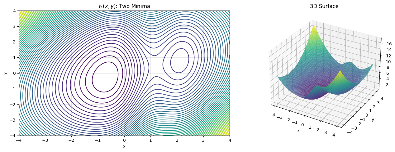
The problem will become more frequent if we are dealing with a function with multiple variables. We will alway get stuck in a local minima. It turns out the previous optimization techniques do not give us the reliable solution. What shall we do?
Brute force methods#
Since the gradient based methods is no longer reliable for the case of multiple minima. We shall return to the more strightforward method.
From the first look, one might immediately come up with two simple ideas:
Grid based search, set a very fine resolution in x-y space, and then evalute the function on each grid
Random sampling, simply generate a lot of (x,y) points, and take the minimum values from all attempts
# Grid search
def grid_search(N):
    x_min, x_max = -4, 4
    y_min, y_max = -4, 4
    minf = f2([x_min,y_min])
    #---to complete-----#
    grid_x = np.linspace(x_min, x_max, N)
    grid_y = np.linspace(y_min, y_max, N)

    f_values = []
    for x in grid_x:
        for y in grid_y:
            f_values.append(f2([x,y]))

    minf = min(f_values)
    #---to complete-----#
    return minf

print (grid_search(20))
0.3903937160062407
# Random search
def random_search(N):
    x_min, x_max = -4, 4
    y_min, y_max = -4, 4
    minf = f2([x_min,y_min])
    #---to complete-----#
    grid_x = np.random.uniform(x_min, x_max, N)
    grid_y = np.random.uniform(y_min, y_max, N)

    f_values = []
    for x in grid_x:
        for y in grid_y:
            f_values.append(f2([x,y]))

    minf = min(f_values)

    #---to complete-----#
    return minf

random_search(100)
np.float64(0.40101879239679317)
Mixed stratergy#
From the above run, one might find that a more effective way as follow,
1, randomly select a point
2, perform a local optimization on each point
This methods would simply take the advantages of both sides, will outperform than all previous methods. In fact, this idea has been largely used nowadays in many fields.
# Mixed Random search

def random_search2(N):
    x_min, x_max = -4, 4
    y_min, y_max = -4, 4
    minf = f2([x_min,y_min])
    #---to complete-----#
    grid_x = np.random.uniform(x_min, x_max, N)
    grid_y = np.random.uniform(y_min, y_max, N)

    f_values = []
    for x in grid_x:
        for y in grid_y:
            res = minimize(f2, [x,y], method='bfgs', tol=1e-4, options={'disp': False})
            f_values.append(res['fun'])

    minf = min(f_values)

    #---to complete-----#
    return minf

for _ in range(10):
    print (random_search2(5))
0.3878588684766304
0.38785886847310447
0.387858868473117
0.38785886847340567
0.3878588684731093
0.38785886847317597
0.3878588684731554
0.3878588684731402
0.38785886847312206
0.3878588684731119
The Exponential Growth Problem#
In high dimensions, the number of local minima grows exponentially.
For example:
1D: 3–5 local minima
3D: dozens to hundreds
100D (typical in molecular optimization): astronomically many
Conclusion: We need methods that can escape local minima.
Lennard-Jones Clusters: Our Running Example#
A Lennard-Jones cluster is a set of N atoms arranged in 3D space to minimize the total interaction energy.
Relevance: Ubiquitous in molecular dynamics, cluster chemistry, materials science
Challenge: Finding the global minimum is NP-hard; known only for small N (N ≤ ~20)
Beauty: Simple energy function, but rich optimization landscape
We’ll use LJ7 and LJ13 throughout L17–L19.
Section II: Lennard-Jones Clusters#
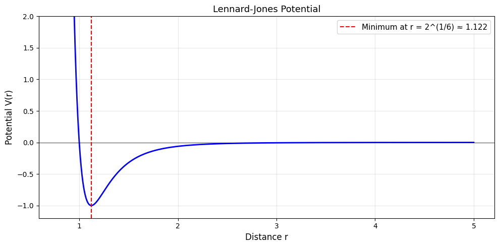
Lennard-Jones Potential#
The pairwise LJ potential between two atoms at distance \(r\) is:
\(r^{-12}\) term: Hard-core repulsion (atoms can’t overlap)
\(r^{-6}\) term: Van der Waals attraction
Minimum: at \(r = 2^{1/6} \approx 1.122\), where \(V = -1\)
def LJ(r):
    'Lennard-Jones potential between two atoms at distance r'

    return 4*(1/r**12 - 1/r**6)

# Plot LJ potential
r = np.linspace(0.8, 5, 500)
V = LJ(r)

plt.figure(figsize=(10, 5))
plt.plot(r, V, 'b-', linewidth=2)
plt.axhline(0, color='k', linestyle='-', linewidth=0.5)
plt.axvline(2**(1/6), color='r', linestyle='--', linewidth=1.5, label=f'Minimum at r = 2^(1/6) ≈ {2**(1/6):.3f}')
plt.xlabel('Distance r', fontsize=12)
plt.ylabel('Potential V(r)', fontsize=12)
plt.title('Lennard-Jones Potential', fontsize=13)
plt.grid(True, alpha=0.3)
plt.legend(fontsize=11)
plt.ylim([-1.2, 2])
plt.tight_layout()
plt.show()
def total_energy(positions):
    '''Total LJ energy for a cluster
    positions: 1D array [x1, y1, z1, x2, y2, z2, ...]'''
    E = 0
    # code
    N_atom = int(len(positions) / 3)
    for i in range(N_atom-1):
        for j in range(i+1, N_atom):
            pos1 = positions[i*3:(i+1)*3]
            pos2 = positions[j*3:(j+1)*3]
            dist = np.linalg.norm(pos1-pos2)
            E += LJ(dist)
    return E

def init_pos(N, L=5):
    'Initialize random positions in a box of side length L'
    return L * np.random.random_sample((N * 3,))
# Demo: random LJ7 cluster
N_atom = 6
pos_random = init_pos(N_atom)
E_random = total_energy(pos_random)

print(f'LJ{N_atom} Cluster:')
print(f'Number of atoms: {N_atom}')
print(f'Number of coordinates: {len(pos_random)}')
print(f'Number of pairwise interactions: {N_atom*(N_atom-1)//2}')
print(f'Energy of random configuration: {E_random:.6f}')
LJ6 Cluster:
Number of atoms: 6
Number of coordinates: 18
Number of pairwise interactions: 15
Energy of random configuration: 76240.793652
# Local optimization with CG
res_cg = minimize(total_energy, pos_random, method='CG', tol=1e-4)
E_cg = res_cg.fun
pos_cg = res_cg.x

print(f'\nAfter CG local optimization:')
print(f'Energy: {E_cg:.6f}')
print(f'Improvement: {E_random - E_cg:.6f}')
After CG local optimization:
Energy: -12.302928
Improvement: 76253.096579
# Multiple random-start local optimization (20 tries)
N_trials = 30
energies = []

for trial in range(N_trials):
    pos_init = init_pos(N_atom)
    res = minimize(total_energy, pos_init, method='CG', tol=1e-4)
    energies.append(res.fun)

energies = np.array(energies)

print(f'Results from {N_trials} random-start CG optimizations:')
print(f'Best energy found: {np.min(energies):.6f}')
print(f'Worst energy found: {np.max(energies):.6f}')
print(f'Mean energy: {np.mean(energies):.6f}')
print(f'Std dev: {np.std(energies):.6f}')
print(f'Known global minimum (Cambridge DB): -16.505384')
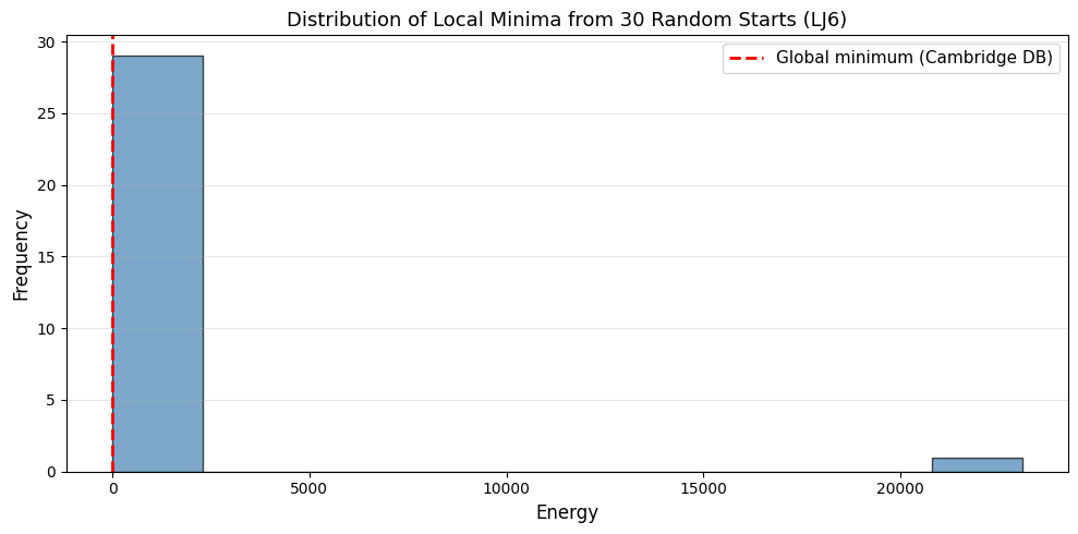
Results from 30 random-start CG optimizations:
Best energy found: -12.712062
Worst energy found: 23097.717242
Mean energy: 758.327537
Std dev: 4148.320863
Known global minimum (Cambridge DB): -16.505384
# Histogram of local minima energies
plt.figure(figsize=(10, 5))
plt.hist(energies, bins=10, edgecolor='black', alpha=0.7, color='steelblue')
plt.axvline(-16.505384, color='r', linestyle='--', linewidth=2, label='Global minimum (Cambridge DB)')
plt.xlabel('Energy', fontsize=12)
plt.ylabel('Frequency', fontsize=12)
plt.title(f'Distribution of Local Minima from {N_trials} Random Starts (LJ{N_atom})', fontsize=13)
plt.legend(fontsize=11)
plt.grid(True, alpha=0.3, axis='y')
plt.tight_layout()
plt.show()
#below are some reference values from Cambridge Cluster database,
#https://doye.chem.ox.ac.uk/jon/structures/LJ/tables.150.html
#please try to download some values from there and check if the results are consistent

#pos =np.array([  -0.3616353090,        0.0439914505,        0.5828840628,
#                  0.2505889242,        0.6193583398,       -0.1614607010,
#                 -0.4082757926,       -0.2212115329,       -0.5067996704,
#                  0.5193221773,       -0.4421382574,        0.08537630870])
pos =np.array([ -0.2604720088,        0.7363147287,        0.4727061929,
                0.2604716550,       -0.7363150782,       -0.4727063011,
               -0.4144908003,       -0.3652598516,        0.3405559620,
               -0.1944131041,        0.2843471802,       -0.5500413671,
                0.6089042582,        0.0809130209,        0.2094855133])

# pos = np.array([ 0.7430002202,        0.2647603899,       -0.0468575389,
#                 -0.7430002647,       -0.2647604843,        0.0468569750,
#                  0.1977276118,       -0.4447220146,        0.6224700350,
#                 -0.1977281310,        0.4447221826,       -0.6224697723,
#                 -0.1822009635,        0.5970484122,        0.4844363476,
#                  0.1822015272,       -0.5970484858,       -0.4844360463])
print (total_energy(pos))
-9.103852415681365
Visulization of the LJ clusters#
ASE package is required: the installation can be done via ‘pip install ase’ command
!pip install ase
Requirement already satisfied: ase in /usr/local/lib/python3.12/dist-packages (3.28.0)
Requirement already satisfied: numpy>=1.21.6 in /usr/local/lib/python3.12/dist-packages (from ase) (2.0.2)
Requirement already satisfied: scipy>=1.8.1 in /usr/local/lib/python3.12/dist-packages (from ase) (1.16.3)
Requirement already satisfied: matplotlib>=3.5.2 in /usr/local/lib/python3.12/dist-packages (from ase) (3.10.0)
Requirement already satisfied: contourpy>=1.0.1 in /usr/local/lib/python3.12/dist-packages (from matplotlib>=3.5.2->ase) (1.3.3)
Requirement already satisfied: cycler>=0.10 in /usr/local/lib/python3.12/dist-packages (from matplotlib>=3.5.2->ase) (0.12.1)
Requirement already satisfied: fonttools>=4.22.0 in /usr/local/lib/python3.12/dist-packages (from matplotlib>=3.5.2->ase) (4.62.1)
Requirement already satisfied: kiwisolver>=1.3.1 in /usr/local/lib/python3.12/dist-packages (from matplotlib>=3.5.2->ase) (1.5.0)
Requirement already satisfied: packaging>=20.0 in /usr/local/lib/python3.12/dist-packages (from matplotlib>=3.5.2->ase) (26.0)
Requirement already satisfied: pillow>=8 in /usr/local/lib/python3.12/dist-packages (from matplotlib>=3.5.2->ase) (11.3.0)
Requirement already satisfied: pyparsing>=2.3.1 in /usr/local/lib/python3.12/dist-packages (from matplotlib>=3.5.2->ase) (3.3.2)
Requirement already satisfied: python-dateutil>=2.7 in /usr/local/lib/python3.12/dist-packages (from matplotlib>=3.5.2->ase) (2.9.0.post0)
Requirement already satisfied: six>=1.5 in /usr/local/lib/python3.12/dist-packages (from python-dateutil>=2.7->matplotlib>=3.5.2->ase) (1.17.0)
#Visulization of the LJ clusters
#ASE package is required: the installation can be done via 'pip install ase' command
from ase.visualize import view
from ase import Atoms
pos =np.array([ -0.2604720088,        0.7363147287,        0.4727061929,
                0.2604716550,       -0.7363150782,       -0.4727063011,
               -0.4144908003,       -0.3652598516,        0.3405559620,
               -0.1944131041,        0.2843471802,       -0.5500413671,
                0.6089042582,        0.0809130209,        0.2094855133])

N=5
cluster = Atoms('N'+str(N), positions=np.reshape(pos*2.0,[N,3]))

view(cluster, viewer='x3d') #view it from jupyter notebook
# view(cluster, viewer='ase') #view it from pop-up ase visualizer
N=12
pos = init_pos(N,L=5)
cluster = Atoms('N'+str(N), positions=np.reshape(pos*2.0,[N,3]))

view(cluster, viewer='x3d') #view it from jupyter notebook
Section III: Simulated Annealing on LJ Clusters#
Simulated Annealing (SA): The Idea#
Inspired by: Annealing in metallurgy (heating and slow cooling to reach low-energy states).
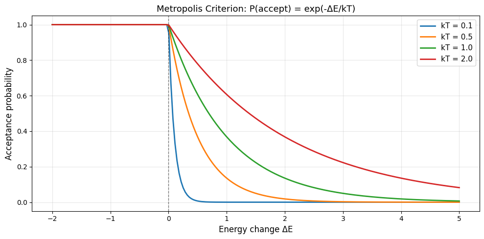
Key insight: At temperature \(T\), accept a move with probability:
where:
\(\Delta E = E_{\text{new}} - E_{\text{old}}\) (energy change)
\(k_B T\) = temperature-like parameter controlling exploration
Strategy: Start hot (accept bad moves), cool down (become selective).
Metropolis Acceptance Probability#
This is the Metropolis criterion (same as HW6!).
# Plot Metropolis acceptance probability for various temperatures
dE_range = np.linspace(-2, 5, 200)
temperatures = [0.1, 0.5, 1.0, 2.0]

plt.figure(figsize=(10, 5))
for T in temperatures:
    prob = np.exp(-np.maximum(0, dE_range) / T)
    plt.plot(dE_range, prob, linewidth=2, label=f'kT = {T}')

plt.axvline(0, color='k', linestyle='--', linewidth=1, alpha=0.5)
plt.xlabel('Energy change ΔE', fontsize=12)
plt.ylabel('Acceptance probability', fontsize=12)
plt.title('Metropolis Criterion: P(accept) = exp(-ΔE/kT)', fontsize=13)
plt.grid(True, alpha=0.3)
plt.legend(fontsize=11)
plt.tight_layout()
plt.show()
SA v1: Basic Simulated Annealing (Fixed Temperature)#
First, let’s implement the simplest version with constant temperature.
def simulated_annealing_v1(N_atom, Max_iteration=1000, kT=1.0):
    'Simulated Annealing (fixed temperature)'
    pos_now = init_pos(N_atom)
    obj_now = total_energy(pos_now)

    best_pos = pos_now.copy()
    best_eng = obj_now

    eng_hist = [obj_now]

    for i in range(Max_iteration):
        # Random step
        step = (np.random.random(len(pos_now)) - 0.5) * 2  # step in [-1, 1]
        pos_new = pos_now + step
        obj_new = total_energy(pos_new)

        # Metropolis acceptance
        dE = obj_new - obj_now
        if dE < 0 or np.random.random() < np.exp(-dE / kT):
            pos_now = pos_new
            obj_now = obj_new

        # Track best
        if obj_now < best_eng:
            best_eng = obj_now
            best_pos = pos_now.copy()

        eng_hist.append(obj_now)

    return best_pos, best_eng, eng_hist
# Test SA v1 on LJ7
np.random.seed(42)
best_pos_v1, best_eng_v1, eng_hist_v1 = simulated_annealing_v1(7, Max_iteration=5000, kT=1.0)

print(f'SA v1 on LJ7 (fixed T=1.0):')
print(f'Best energy: {best_eng_v1:.6f}')
print(f'Known global minimum: -16.505384')
print(f'Gap: {best_eng_v1 - (-16.505384):.6f}')
SA v1 on LJ7 (fixed T=1.0):
Best energy: -1.675530
Known global minimum: -16.505384
Gap: 14.829854
SA v2: SA + Local Optimization (Basin Hopping Style)#
At each step, perform a random walk followed by local optimization. This is the bridge to Basin Hopping.
def simulated_annealing_v2(N_atom, Max_iteration=100, kT=1.0, step_size=0.5):
    'SA + local optimization at each step (basin hopping style)'
    pos_now = init_pos(N_atom)
    res = minimize(total_energy, pos_now, method='CG', tol=1e-4)
    pos_now = res.x
    obj_now = res.fun

    best_pos = pos_now.copy()
    best_eng = obj_now
    eng_hist = [obj_now]

    for i in range(Max_iteration):
        # Random perturbation
        pos_new = pos_now + step_size * (np.random.random(len(pos_now)) - 0.5)

        # Local optimization
        res = minimize(total_energy, pos_new, method='CG', tol=1e-4)
        pos_new = res.x
        obj_new = res.fun

        # Metropolis acceptance
        dE = obj_new - obj_now
        if dE < 0 or np.random.random() < np.exp(-dE / kT):
            pos_now = pos_new
            obj_now = obj_new

        # Track best
        if obj_now < best_eng:
            best_eng = obj_now
            best_pos = pos_now.copy()

        eng_hist.append(obj_now)

    return best_pos, best_eng, eng_hist
# Test SA v2 on LJ7
np.random.seed(42)
best_pos_v2, best_eng_v2, eng_hist_v2 = simulated_annealing_v2(9, Max_iteration=100, kT=1.0, step_size=0.5)

print(f'SA v2 on LJ7 (with local optimization):')
print(f'Best energy: {best_eng_v2:.6f}')
print(f'Known global minimum: -16.505384')
print(f'Gap: {best_eng_v2 - (-16.505384):.6f}')
SA v2 on LJ7 (with local optimization):
Best energy: -24.113360
Known global minimum: -16.505384
Gap: -7.607976
SA v3: SA with Geometric Cooling Schedule#
The key to SA is the cooling schedule: how to reduce temperature over time.
Geometric cooling#
where:
\(T_0\) = initial temperature
\(\alpha\) = cooling rate (e.g., 0.95)
\(n\) = iteration number
This exponentially decays the temperature, allowing early exploration and late exploitation.
def simulated_annealing_v3(N_atom, Max_iteration=200, T0=2.0, alpha=0.95, step_size=0.5):
    'SA with geometric cooling schedule'
    pos_now = init_pos(N_atom)
    res = minimize(total_energy, pos_now, method='CG', tol=1e-4)
    pos_now = res.x
    obj_now = res.fun

    best_pos = pos_now.copy()
    best_eng = obj_now
    eng_hist = [obj_now]
    T_hist = [T0]

    for i in range(Max_iteration):
        T = T0 * (alpha ** i)

        # Random perturbation
        pos_new = pos_now + step_size * (np.random.random(len(pos_now)) - 0.5)

        # Local optimization
        res = minimize(total_energy, pos_new, method='CG', tol=1e-4)
        pos_new = res.x
        obj_new = res.fun

        # Metropolis acceptance
        dE = obj_new - obj_now
        if dE < 0 or np.random.random() < np.exp(-dE / T):
            pos_now = pos_new
            obj_now = obj_new

        # Track best
        if obj_now < best_eng:
            best_eng = obj_now
            best_pos = pos_now.copy()

        eng_hist.append(obj_now)
        T_hist.append(T)

    return best_pos, best_eng, eng_hist, T_hist
# Test SA v3 on LJ7
np.random.seed(42)
best_pos_v3, best_eng_v3, eng_hist_v3, T_hist_v3 = simulated_annealing_v3(
    7, Max_iteration=200, T0=2.0, alpha=0.95, step_size=0.5
)

print(f'SA v3 on LJ7 (geometric cooling, T0=2.0, alpha=0.95):')
print(f'Best energy: {best_eng_v3:.6f}')
print(f'Known global minimum: -16.505384')
print(f'Gap: {best_eng_v3 - (-16.505384):.6f}')
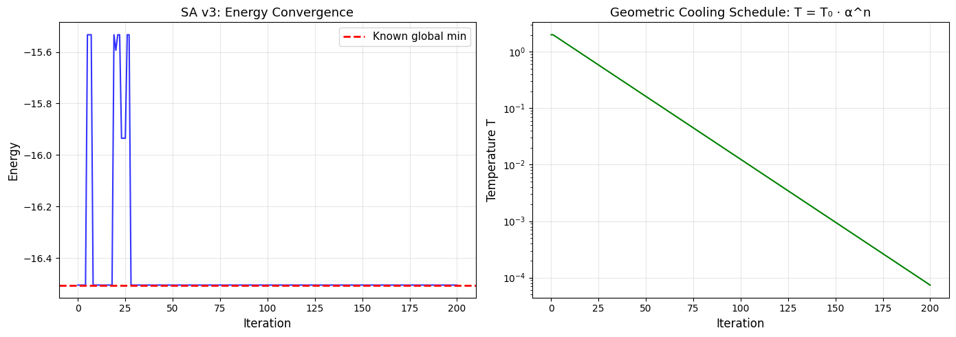
SA v3 on LJ7 (geometric cooling, T0=2.0, alpha=0.95):
Best energy: -16.505384
Known global minimum: -16.505384
Gap: -0.000000
# Plot energy and temperature history
fig, (ax1, ax2) = plt.subplots(1, 2, figsize=(14, 5))

# Energy vs iteration
ax1.plot(eng_hist_v3, 'b-', linewidth=1.5, alpha=0.8)
ax1.axhline(-16.505384, color='r', linestyle='--', linewidth=2, label='Known global min')
ax1.set_xlabel('Iteration', fontsize=12)
ax1.set_ylabel('Energy', fontsize=12)
ax1.set_title('SA v3: Energy Convergence', fontsize=13)
ax1.grid(True, alpha=0.3)
ax1.legend(fontsize=11)

# Temperature vs iteration
ax2.plot(T_hist_v3, 'g-', linewidth=1.5)
ax2.set_xlabel('Iteration', fontsize=12)
ax2.set_ylabel('Temperature T', fontsize=12)
ax2.set_title('Geometric Cooling Schedule: T = T₀ · α^n', fontsize=13)
ax2.grid(True, alpha=0.3)
ax2.set_yscale('log')

plt.tight_layout()
plt.show()
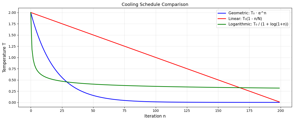
# Compare three cooling schedules
n_iter = 200
T0 = 2.0
n = np.arange(n_iter)

# Geometric
T_geom = T0 * (0.95 ** n)

# Linear
T_lin = T0 * (1 - n / n_iter)
T_lin = np.maximum(T_lin, 0)  # avoid negative

# Logarithmic
T_log = T0 / (1 + np.log(1 + n))

plt.figure(figsize=(12, 5))
plt.plot(n, T_geom, 'b-', linewidth=2, label='Geometric: T₀ · α^n')
plt.plot(n, T_lin, 'r-', linewidth=2, label='Linear: T₀(1 - n/N)')
plt.plot(n, T_log, 'g-', linewidth=2, label='Logarithmic: T₀ / (1 + log(1+n))')
plt.xlabel('Iteration n', fontsize=12)
plt.ylabel('Temperature T', fontsize=12)
plt.title('Cooling Schedule Comparison', fontsize=13)
plt.legend(fontsize=11)
plt.grid(True, alpha=0.3)
plt.tight_layout()
plt.show()
Section IV: Basin Hopping#
The Idea: Transforming the Landscape#
Basin hopping is a clever trick:
Instead of optimizing \(f(\mathbf{x})\) directly, we create a new function:
This transforms the jagged landscape into a staircase:
Each basin (region around a local minimum) becomes a single point
The stalactites (local variations) disappear
Metropolis sampling now hops between basins, not within them
Algorithm:
Random perturbation of current position
Local optimization (minimize to nearby local minimum)
Metropolis acceptance based on the minimized energy
Accept or reject the whole basin
This is much more efficient than raw SA!
def basin_hopping_custom(N_atom, Max_iteration=100, kT=0.5, step_size=0.5):
    'Custom Basin Hopping implementation'
    pos_now = init_pos(N_atom)
    res = minimize(total_energy, pos_now, method='CG', tol=1e-4)
    pos_now = res.x
    obj_now = res.fun

    best_pos = pos_now.copy()
    best_eng = obj_now
    eng_hist = [obj_now]
    accept_hist = [1]  # track acceptance

    for i in range(Max_iteration):
        # Random perturbation
        pos_new = pos_now + step_size * (np.random.random(len(pos_now)) - 0.5)

        # Local optimization
        res = minimize(total_energy, pos_new, method='CG', tol=1e-4)
        pos_new = res.x
        obj_new = res.fun

        # Metropolis acceptance (on the local minimum energies)
        dE = obj_new - obj_now
        if dE < 0 or np.random.random() < np.exp(-dE / kT):
            pos_now = pos_new
            obj_now = obj_new
            accept = 1
        else:
            accept = 0

        # Track best
        if obj_now < best_eng:
            best_eng = obj_now
            best_pos = pos_now.copy()

        eng_hist.append(obj_now)
        accept_hist.append(accept)

    accept_rate = np.mean(accept_hist)
    return best_pos, best_eng, eng_hist, accept_rate
# Basin Hopping on LJ7
np.random.seed(42)
bh_pos, bh_eng, bh_hist, bh_accept = basin_hopping_custom(7, Max_iteration=100, kT=0.5, step_size=0.5)

print(f'Basin Hopping on LJ7:')
print(f'Best energy: {bh_eng:.6f}')
print(f'Known global minimum: -16.505384')
print(f'Gap: {bh_eng - (-16.505384):.6f}')
print(f'Acceptance rate: {bh_accept:.1%}')
Basin Hopping on LJ7:
Best energy: -16.505384
Known global minimum: -16.505384
Gap: -0.000000
Acceptance rate: 90.1%
# Basin Hopping on LJ9
np.random.seed(42)
bh_pos_9, bh_eng_9, bh_hist_9, bh_accept_9 = basin_hopping_custom(9, Max_iteration=200, kT=1.0, step_size=0.5)

print(f'\nBasin Hopping on LJ9:')
print(f'Best energy: {bh_eng_9:.6f}')
print(f'Known global minimum: 	-24.113360')
print(f'Gap: {bh_eng_9 - (-24.113360):.6f}')
print(f'Acceptance rate: {bh_accept_9:.1%}')
Basin Hopping on LJ9:
Best energy: -24.113360
Known global minimum: 	-24.113360
Gap: -0.000000
Acceptance rate: 90.0%
Section V: Summary#
Key Takeaways#
Local methods fail in high-dimensional, multi-modal problems
Simulated Annealing:
Uses Metropolis criterion to escape local minima
Requires cooling schedule tuning
Can be slow for difficult problems
Basin Hopping is often superior:
Transforms rough landscape into staircase of basins
Perturb → minimize → accept (accept/reject entire basins)
Much more efficient than raw Metropolis random walk
For Lennard-Jones clusters:
Basin Hopping finds global minima reliably
Cambridge Cluster Database has known global minima for reference
Scaling: grows harder exponentially with N atoms
What’s Next? (L18–L19)#
Evolutionary Algorithms: Genetic Algorithms
Particle Swarm Optimization: Population-based, inspired by bird flocking
Hybrid methods: Combine global search with local polishing