Lecture 18: Global Optimization II

Genetic Algorithms, Differential Evolution & Particle Swarm Optimization

Context: L17 covered Simulated Annealing and Basin Hopping for LJ cluster optimization. Today we extend to population-based methods that explore MANY solutions simultaneously.

import numpy as np
import matplotlib.pyplot as plt
from scipy.optimize import minimize, differential_evolution
from scipy.spatial.distance import pdist, squareform
from random import sample
from time import time
import warnings
warnings.filterwarnings('ignore')

np.random.seed(42)
plt.style.use('seaborn-v0_8-darkgrid')
%matplotlib inline

Why Population-Based Methods?

Single-point methods (SA, Basin Hopping):

• Explore ONE solution at a time

• Sequential improvement toward local minima

• Limited parallelism

Population-based methods (GA, DE, PSO):

• Maintain a POPULATION of solutions simultaneously

• Explore diverse regions of the landscape in parallel

• Information sharing between solutions → better convergence

• Natural parallelization across population members

• Inspired by nature: evolution, physics, animal behavior

Trade-offs:

• Higher computational cost per generation (but parallel)

• Fewer function evaluations per solution (wider search)

• Better for high-dimensional, multimodal problems

def LJ(r):
    """Lennard-Jones pair potential."""
    r6 = r**6
    r12 = r6*r6
    return 4*(1/r12 - 1/r6)

def total_energy(positions):
    """Compute total LJ energy of atomic cluster.
    positions: flat array [x1,y1,z1, x2,y2,z2, ...]
    """
    E = 0
    N_atom = int(len(positions)/3)
    for i in range(N_atom-1):
        for j in range(i+1, N_atom):
            pos1 = positions[i*3:(i+1)*3]
            pos2 = positions[j*3:(j+1)*3]
            dist = np.linalg.norm(pos1-pos2)
            E += LJ(dist)
    return E

def init_pos(N, L=5):
    """Initialize N atoms randomly in a cube [-L/2, L/2]^3."""
    return L*np.random.random_sample((N*3,)) - L/2

def init_population(pop_size, N_atom, L=5):
    """Initialize a population of random cluster configurations."""
    return [init_pos(N_atom, L) for _ in range(pop_size)]

Section II: Genetic Algorithms (GA)

Biological Analogy

Concept	Biology	Optimization
Individual	Organism	Cluster configuration
Gene	DNA sequence	Position coordinate
Population	Species	Set of solutions
Fitness	Survival/reproduction ability	Negative energy (lower = better)
Selection	Natural selection	Tournament/fitness-based
Crossover	Sexual reproduction	Combine two parents
Mutation	Genetic variation	Random perturbation

GA Cycle

1. Evaluate: Compute fitness of all individuals

2. Select: Choose parents based on fitness (tournament selection)

3. Crossover: Blend parent solutions to create offspring

4. Mutate: Introduce random variation

5. Replace: Update population (elitism: keep best)

6. Repeat: Until convergence or max generations

def selTournament(fitness, factor=0.35):
    """Select one individual via tournament selection.
    
    Draw a random sample of size factor*len(fitness),
    return the index of the best (lowest fitness) in that sample.
    """
    IDs = sample(list(range(len(fitness))), int(len(fitness)*factor))
    min_fit = np.argmin(np.array(fitness)[IDs])
    return IDs[min_fit]

def crossover(cluster, fitness):
    """Arithmetic crossover: blend two tournament-selected parents.
    
    child = frac * parent1 + (1-frac) * parent2
    where frac is random in [0,1].
    """
    id1 = selTournament(fitness)
    while True:
        id2 = selTournament(fitness)
        if id2 != id1:
            break
    frac = np.random.random()
    return cluster[id1] * frac + cluster[id2] * (1 - frac)

def mutation(cluster, fitness, kT=0.5):
    """Gaussian mutation: perturb a tournament-selected individual.
    
    new_positions = parent + (random - 0.5) * kT
    kT controls mutation strength (temperature-like parameter).
    """
    idx = selTournament(fitness)
    cluster0 = cluster[idx].copy()
    disp = np.random.random_sample((len(cluster0),)) - 0.5
    return cluster0 + disp * kT

def local_optimize(cluster, method='CG', maxiter=50):
    """Refine each cluster in the population using local optimization.
    
    This is a hybrid GA+local search approach (Lamarckian evolution).
    Each individual is locally optimized before evaluation.
    """
    optimized = []
    fitness = []
    for pos in cluster:
        res = minimize(total_energy, pos, method=method, 
                      options={'maxiter': maxiter}, tol=1e-4)
        optimized.append(res.x)
        fitness.append(res.fun)
    return optimized, np.array(fitness)

def GA(N_atom=10, n_gen=10, pop_size=10, ratio=0.7, local_opt=True):
    """Genetic Algorithm for cluster optimization.
    
    Parameters:
    -----------
    N_atom : int
        Number of atoms in cluster
    n_gen : int
        Number of generations
    pop_size : int
        Population size
    ratio : float
        Fraction of offspring from crossover (rest from mutation)
    local_opt : bool
        Whether to locally optimize each individual
    
    Returns:
    --------
    cluster : list of arrays
        Final population
    fitness : ndarray
        Final fitness values
    history : list
        Best fitness at each generation
    """
    history = []
    t0 = time()
    
    for gen in range(n_gen):
        # Initialize population
        if gen == 0:
            cluster = init_population(pop_size, N_atom)
        
        # Evaluate and (optionally) refine
        if local_opt:
            cluster, fitness = local_optimize(cluster)
        else:
            fitness = np.array([total_energy(pos) for pos in cluster])
        
        best_e = np.min(fitness)
        history.append(best_e)
        print(f'Gen {gen:2d}: best_E = {best_e:8.4f}')
        
        # Create next generation
        new_cluster = []
        for j in range(pop_size):
            if j < int(ratio * pop_size):
                # Crossover
                new_cluster.append(crossover(cluster, fitness))
            else:
                # Mutation
                new_cluster.append(mutation(cluster, fitness, kT=0.5))
        cluster = new_cluster
    
    elapsed = time() - t0
    print(f'Total time: {elapsed:.2f} s')
    
    return cluster, fitness, history

# Run GA on LJ7 (heptamer)
print('='*50)
print('Genetic Algorithm on LJ7')
print('='*50)
cluster7_ga, fitness7_ga, hist7_ga = GA(N_atom=7, n_gen=15, pop_size=20, 
                                         ratio=0.7, local_opt=True)

==================================================
Genetic Algorithm on LJ7
==================================================
Gen  0: best_E = -13.9151
Gen  1: best_E = -16.5054
Gen  2: best_E = -16.5054
Gen  3: best_E = -16.5054
Gen  4: best_E = -16.5054
Gen  5: best_E = -16.5054
Gen  6: best_E = -16.5054
Gen  7: best_E = -16.5054
Gen  8: best_E = -16.5054
Gen  9: best_E = -16.5054
Gen 10: best_E = -16.5054
Gen 11: best_E = -16.5054
Gen 12: best_E = -16.5054
Gen 13: best_E = -16.5054
Gen 14: best_E = -16.5054
Total time: 17.25 s

print('\n' + '='*50)
print('Genetic Algorithm on LJ13')
print('='*50)
cluster13_ga, fitness13_ga, hist13_ga = GA(N_atom=13, n_gen=20, pop_size=30, 
                                            ratio=0.7, local_opt=True)

==================================================
Genetic Algorithm on LJ13
==================================================
Gen  0: best_E = -29.7890
Gen  1: best_E = -38.2558
Gen  2: best_E = -40.6155
Gen  3: best_E = -44.3268
Gen  4: best_E = -44.3268
Gen  5: best_E = -44.3268
Gen  6: best_E = -44.3268
Gen  7: best_E = -44.3268
Gen  8: best_E = -44.3268
Gen  9: best_E = -44.3268
Gen 10: best_E = -44.3268
Gen 11: best_E = -44.3268
Gen 12: best_E = -44.3268
Gen 13: best_E = -44.3268
Gen 14: best_E = -44.3268
Gen 15: best_E = -44.3268
Gen 16: best_E = -44.3268
Gen 17: best_E = -44.3268
Gen 18: best_E = -44.3268
Gen 19: best_E = -44.3268
Total time: 160.57 s

fig, axes = plt.subplots(1, 2, figsize=(14, 5))

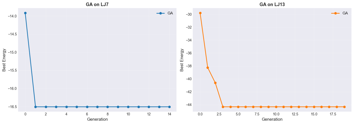
axes[0].plot(hist7_ga, 'o-', linewidth=2, markersize=6, label='GA')
axes[0].set_xlabel('Generation', fontsize=12)
axes[0].set_ylabel('Best Energy', fontsize=12)
axes[0].set_title('GA on LJ7', fontsize=13, fontweight='bold')
axes[0].grid(True, alpha=0.3)
axes[0].legend(fontsize=11)

axes[1].plot(hist13_ga, 'o-', linewidth=2, markersize=6, color='tab:orange', label='GA')
axes[1].set_xlabel('Generation', fontsize=12)
axes[1].set_ylabel('Best Energy', fontsize=12)
axes[1].set_title('GA on LJ13', fontsize=13, fontweight='bold')
axes[1].grid(True, alpha=0.3)
axes[1].legend(fontsize=11)

plt.tight_layout()
plt.show()

Parameter Sensitivity Analysis

Population size: Larger populations explore more broadly, but slower convergence per generation. Typical range: 15-50 for continuous optimization.

Crossover ratio: Higher ratio → more exploration (blending), lower ratio → more mutation (diversity). Typical range: 0.6-0.9.

Mutation strength (kT): Controls perturbation magnitude. Too small → premature convergence; too large → chaos. Adaptive approaches: reduce kT as fitness improves (cooling schedule).

Local optimization: Hybrid GA (Lamarckian evolution) refines individuals before selection. Cost: higher per-generation, but typically faster overall convergence. Classical GA (Darwinian) skips local opt: faster per-gen but slower asymptotic convergence.

print('GA Results Summary:')
print(f'LJ7:  best_E = {min(hist7_ga):.4f} (gens: {len(hist7_ga)})')
print(f'LJ13: best_E = {min(hist13_ga):.4f} (gens: {len(hist13_ga)})')
print()
print('Known minima (for reference):')
print('LJ7:  E ~ -16.505')
print('LJ13: E ~ -44.326')

GA Results Summary:
LJ7:  best_E = -16.5054 (gens: 15)
LJ13: best_E = -44.3268 (gens: 20)

Known minima (for reference):
LJ7:  E ~ -16.505
LJ13: E ~ -44.326

Lamarckian vs Pure GA: The Power of Local Optimization

A Lamarckian GA (also called a memetic algorithm) applies local optimization to each individual after genetic operations. This is analogous to Lamarckian evolution where acquired traits are inherited.

Without local optimization: GA explores the raw energy surface — crossover and mutation produce configurations that may be far from any local minimum. Progress is slow.

With local optimization: Each individual is refined to the nearest local minimum before selection. The GA now searches the space of local minima — dramatically smaller and smoother than the raw landscape.

This is the same insight as Basin Hopping (L17): always compare locally minimized energies.

# Compare GA with and without local optimization on LJ7
print('='*60)
print('GA Comparison: With vs Without Local Optimization')
print('='*60)

# Without local optimization (pure GA)
print('\nPure GA (no local opt):')
np.random.seed(42)
_, _, hist7_ga_pure = GA(N_atom=7, n_gen=15, pop_size=20, 
                         ratio=0.7, local_opt=False)

# With local optimization (Lamarckian/memetic)
print('\nLamarckian GA (with local opt):')
np.random.seed(42)
_, _, hist7_ga_lamarck = GA(N_atom=7, n_gen=15, pop_size=20, 
                             ratio=0.7, local_opt=True)

# Convergence comparison plot
fig, ax = plt.subplots(figsize=(10, 6))
ax.plot(hist7_ga_pure, 's--', linewidth=2, markersize=7, 
        color='tab:red', label='Pure GA (no local opt)')
ax.plot(hist7_ga_lamarck, 'o-', linewidth=2.5, markersize=7, 
        color='tab:blue', label='Lamarckian GA (with local opt)')
ax.axhline(y=-16.505384, color='black', linestyle=':', linewidth=1.5, 
           label='Known global min (-16.505)')
ax.set_xlabel('Generation', fontsize=13)
ax.set_ylabel('Best Energy', fontsize=13)
ax.set_title('LJ7: Effect of Local Optimization in GA', fontsize=14, fontweight='bold')
ax.legend(fontsize=12)
ax.grid(True, alpha=0.3)
plt.tight_layout()
plt.show()

print(f'\nPure GA final:      {min(hist7_ga_pure):.4f}')
print(f'Lamarckian GA final: {min(hist7_ga_lamarck):.4f}')
print(f'Known global min:    -16.505384')

============================================================
GA Comparison: With vs Without Local Optimization
============================================================

Pure GA (no local opt):
Gen  0: best_E =  -2.9199
Gen  1: best_E =  -5.3837
Gen  2: best_E =  -4.0717
Gen  3: best_E =  -4.5285
Gen  4: best_E =  -4.5565
Gen  5: best_E =  -4.7303
Gen  6: best_E =  -4.8763
Gen  7: best_E =  -4.8776
Gen  8: best_E =  -4.8776
Gen  9: best_E =  -4.8776
Gen 10: best_E =  -4.8776
Gen 11: best_E =  -4.8776
Gen 12: best_E =  -4.8776
Gen 13: best_E =  -4.8776
Gen 14: best_E =  -4.8776
Total time: 0.03 s

Lamarckian GA (with local opt):
Gen  0: best_E = -13.9151
Gen  1: best_E = -16.5054
Gen  2: best_E = -16.5054
Gen  3: best_E = -16.5054
Gen  4: best_E = -16.5054
Gen  5: best_E = -16.5054
Gen  6: best_E = -16.5054
Gen  7: best_E = -16.5054
Gen  8: best_E = -16.5054
Gen  9: best_E = -16.5054
Gen 10: best_E = -16.5054
Gen 11: best_E = -16.5054
Gen 12: best_E = -16.5054
Gen 13: best_E = -16.5054
Gen 14: best_E = -16.5054
Total time: 18.83 s

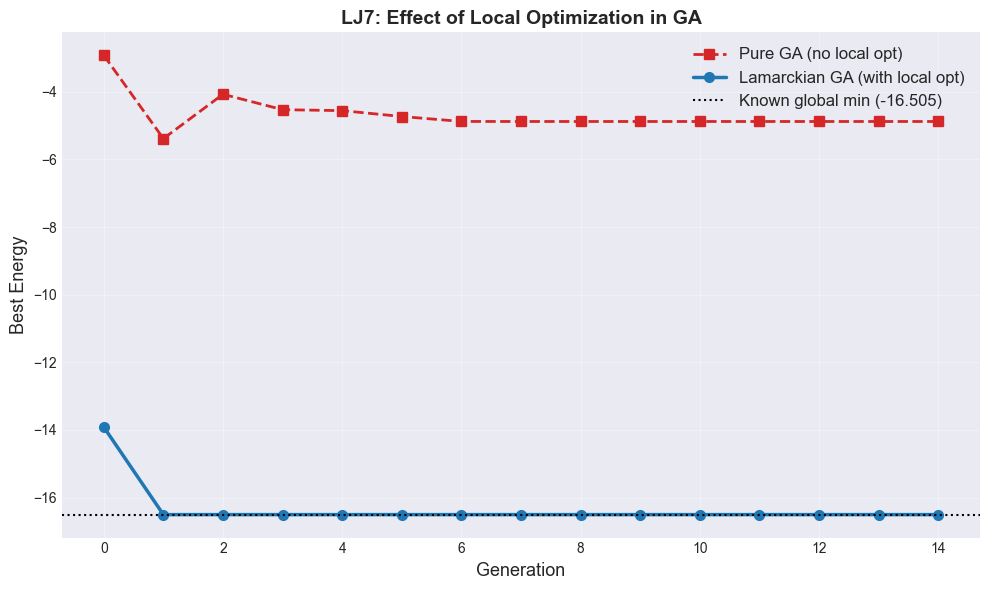
Pure GA final:      -5.3837
Lamarckian GA final: -16.5054
Known global min:    -16.505384

GA vs SA (from L17)

Aspect	GA	SA
Parallelism	Natural (population)	Sequential
Memory	O(pop_size * dim)	O(dim)
Bias	Implicit; selection drives convergence	Temperature schedule
Tuning	Pop size, crossover ratio, mutation	Cooling schedule, accept prob
Scalability	Better for large populations	Better for single-run memory
Convergence	Can plateau (loss of diversity)	Probabilistic guarantee (T→0)

Section III: Differential Evolution (DE)

Core Idea

DE combines mutation based on population variance with crossover and selection.

Key Operators

1. Mutation: For each individual \(\mathbf{x}_i\), create a mutant: $\(\mathbf{v}_i = \mathbf{x}_{r_1} + F \cdot (\mathbf{x}_{r_2} - \mathbf{x}_{r_3})\)\( where \)r_1, r_2, r_3\( are distinct random indices, \)F \in (0, 2)$ is the scaling factor.

2. Crossover: Blend mutant with parent (binomial or exponential): $\(u_i^j = \begin{cases} v_i^j & \text{if } \text{rand} < CR \\ x_i^j & \text{otherwise} \end{cases}\)\( where \)CR \in [0,1]$ is crossover probability.

3. Selection: If \(f(\mathbf{u}) < f(\mathbf{x}_i)\), replace: \(\mathbf{x}_i \leftarrow \mathbf{u}\)

Advantages over GA

• No explicit selection step: Automatic self-adaptation

• Mutation uses population variance: Scales with problem structure

• Fewer hyperparameters: Mainly \(F\) and \(CR\)

• Excellent convergence: Especially for continuous, bounded problems

# scipy.optimize.differential_evolution is a robust, production-grade DE
# We use it directly rather than implementing from scratch

def run_de_scipy(N_atom, bounds_width=3.0, maxiter=200, seed=42):
    """Run scipy's DE on LJ cluster.
    
    Parameters:
    -----------
    N_atom : int
        Number of atoms
    bounds_width : float
        Search bounds: [-bounds_width, bounds_width] per coordinate
    maxiter : int
        Max iterations
    seed : int
        Random seed for reproducibility
    """
    dim = N_atom * 3
    bounds = [(-bounds_width, bounds_width)] * dim
    
    t0 = time()
    result = differential_evolution(total_energy, bounds, maxiter=maxiter, 
                                    seed=seed, workers=1, updating='deferred',
                                    atol=0, tol=1e-7, disp=False)
    elapsed = time() - t0
    
    return result, elapsed

print('='*50)
print('Differential Evolution on LJ7')
print('='*50)
result7_de, t7_de = run_de_scipy(N_atom=7, maxiter=200, seed=42)
print(f'Best energy: {result7_de.fun:.4f}')
print(f'Nfev: {result7_de.nfev}')
print(f'Time: {t7_de:.2f} s')
print(f'Convergence: {"Yes" if result7_de.success else "No"}')

==================================================
Differential Evolution on LJ7
==================================================
Best energy: -16.5054
Nfev: 65097
Time: 3.45 s
Convergence: No

print('\n' + '='*50)
print('Differential Evolution on LJ13')
print('='*50)
result13_de, t13_de = run_de_scipy(N_atom=13, maxiter=300, seed=42)
print(f'Best energy: {result13_de.fun:.4f}')
print(f'Nfev: {result13_de.nfev}')
print(f'Time: {t13_de:.2f} s')
print(f'Convergence: {"Yes" if result13_de.success else "No"}')

==================================================
Differential Evolution on LJ13
==================================================
Best energy: -39.6355
Nfev: 181165
Time: 31.16 s
Convergence: No

# scipy.optimize.differential_evolution tracks fitness in result.func_vals
# For a fair comparison with GA, we approximate from the result object
# A more detailed custom DE would track this explicitly

print('DE converged to:')
print(f'LJ7:  E = {result7_de.fun:.4f}')
print(f'LJ13: E = {result13_de.fun:.4f}')
print()
print('Compare to GA results:')
print(f'GA LJ7:  E = {min(hist7_ga):.4f}')
print(f'GA LJ13: E = {min(hist13_ga):.4f}')

DE converged to:
LJ7:  E = -16.5054
LJ13: E = -39.6355

Compare to GA results:
GA LJ7:  E = -16.5054
GA LJ13: E = -44.3268

# DE + Local Polish: refine DE result with CG
from scipy.optimize import minimize as sp_minimize

print('DE + Local Polish:')
print('='*50)

# Polish LJ7
res7_polished = sp_minimize(total_energy, result7_de.x, method='CG', 
                            options={'maxiter': 200})
print(f'LJ7:  DE alone = {result7_de.fun:.4f}  →  DE+CG = {res7_polished.fun:.4f}')

# Polish LJ13
res13_polished = sp_minimize(total_energy, result13_de.x, method='CG', 
                             options={'maxiter': 200})
print(f'LJ13: DE alone = {result13_de.fun:.4f}  →  DE+CG = {res13_polished.fun:.4f}')

print()
print('Known global minima:')
print(f'LJ7:  -16.505384')
print(f'LJ13: -44.326801')
print()
print('Note: DE+CG polishes to the nearest local minimum,')
print('but DE may not have found the basin of the global minimum.')

DE + Local Polish:
==================================================
LJ7:  DE alone = -16.5054  →  DE+CG = -16.5054
LJ13: DE alone = -39.6355  →  DE+CG = -39.6355

Known global minima:
LJ7:  -16.505384
LJ13: -44.326801

Note: DE+CG polishes to the nearest local minimum,
but DE may not have found the basin of the global minimum.

DE Observations

Strengths:

• Typically finds lower energy than GA in comparable number of function evals

• Self-adaptive scaling (via population variance in mutation)

• Robust across many problem types (no tuning needed)

• Deterministic replacement (simpler than fitness-based selection)

Weaknesses:

• Loses diversity as population converges (no explicit diversity maintenance)

• Fixed population size (unlike GA where we can vary)

When to use DE:

• Continuous optimization with bounds

• High-dimensional problems (D > 50)

• Limited prior knowledge of landscape

# Theory: DE mutation strategy depends on variant
# Standard: DE/rand/1/bin (what scipy uses)
# v_i = x_r1 + F * (x_r2 - x_r3)
# 
# Other variants:
# - DE/best/1: v_i = x_best + F * (x_r1 - x_r2)  [greedy]
# - DE/current-to-best/1: hybrid of both
# 
# Crossover variants:
# - Binomial: independent Bernoulli on each dimension
# - Exponential: contiguous segment from mutant

print('DE Hyperparameters (scipy defaults):')
print('F (scale factor): auto-tuned')
print('CR (crossover prob): 0.7')
print('Population size: 15*dim')
print('Mutation strategy: best1bin')

DE Hyperparameters (scipy defaults):
F (scale factor): auto-tuned
CR (crossover prob): 0.7
Population size: 15*dim
Mutation strategy: best1bin

Local Optimization with DE

DE alone often achieves very good results without local refinement. However, polishing with local optimization (CG, L-BFGS) after DE can sometimes improve the final result.

## Polish DE result with local opt
from scipy.optimize import minimize
res_polished = minimize(total_energy, result.x, method='CG')

This hybrid (DE + local polish) is called memetic algorithms in the literature.

Section IV: Particle Swarm Optimization (PSO)

Swarm Intelligence Inspiration

• Birds flocking, fish schooling: individuals follow simple rules

• Emergent collective behavior: group finds food more efficiently than individuals

• No central control; communication through social influence

PSO Mechanics

Each particle \(i\) has:

• Position: \(\mathbf{x}_i\)

• Velocity: \(\mathbf{v}_i\)

• Personal best: \(\mathbf{p}_i\) (best position found so far)

• Global best: \(\mathbf{g}\) (best position in entire swarm)

Velocity Update Rule

\[\mathbf{v}_i \leftarrow w \mathbf{v}_i + c_1 r_1 (\mathbf{p}_i - \mathbf{x}_i) + c_2 r_2 (\mathbf{g} - \mathbf{x}_i)\]

where:

• \(w\) = inertia weight (0.5-0.9): balance between exploration & exploitation

• \(c_1\) = cognitive/personal coefficient (~1.5): trust in own experience

• \(c_2\) = social/global coefficient (~1.5): trust in swarm information

• \(r_1, r_2\) = random in \([0,1]\)

Position Update Rule

\[\mathbf{x}_i \leftarrow \mathbf{x}_i + \mathbf{v}_i\]

def pso(N_atom, iters=20, pop_size=30, w=0.5, c1=1.5, c2=1.5, 
        local_opt_freq=1, verbose=True):
    """Particle Swarm Optimization for cluster energy minimization.
    
    Parameters:
    -----------
    N_atom : int
        Number of atoms
    iters : int
        Number of PSO iterations
    pop_size : int
        Swarm size
    w : float
        Inertia weight
    c1 : float
        Cognitive coefficient (personal best)
    c2 : float
        Social coefficient (global best)
    local_opt_freq : int
        Frequency of local optimization (every N iterations)
    verbose : bool
        Print progress
    
    Returns:
    --------
    g_best_X : ndarray
        Best position found
    g_best_score : float
        Best energy
    history : list
        Best energy at each iteration
    """
    dim = N_atom * 3
    bounds = 3.0
    
    # Initialize positions and velocities
    X = np.random.uniform(-bounds, bounds, size=(pop_size, dim))
    V = (np.random.random((pop_size, dim)) - 0.5) * 0.3
    
    # Evaluate initial fitness
    scores = np.array([total_energy(x) for x in X])
    
    # Initialize personal and global bests
    p_best_X = X.copy()
    p_best_score = scores.copy()
    g_idx = np.argmin(scores)
    g_best_X = X[g_idx].copy()
    g_best_score = scores[g_idx]
    
    history = [g_best_score]
    t0 = time()
    
    for iteration in range(iters):
        # Optional local refinement every N iterations
        if local_opt_freq > 0 and iteration % local_opt_freq == 0:
            for i in range(pop_size):
                res = minimize(total_energy, X[i], method='CG', 
                             options={'maxiter': 30}, tol=1e-3)
                X[i] = res.x
                scores[i] = res.fun
        
        # Update personal and global bests
        for i in range(pop_size):
            if scores[i] < p_best_score[i]:
                p_best_score[i] = scores[i]
                p_best_X[i] = X[i].copy()
        
        idx = np.argmin(p_best_score)
        if p_best_score[idx] < g_best_score:
            g_best_score = p_best_score[idx]
            g_best_X = p_best_X[idx].copy()
        
        history.append(g_best_score)
        
        if verbose and iteration % 5 == 0:
            print(f'Iter {iteration:2d}: best_E = {g_best_score:8.4f}')
        
        # Velocity and position update
        r1 = np.random.random((pop_size, dim))
        r2 = np.random.random((pop_size, dim))
        
        V = (w * V + 
             c1 * r1 * (p_best_X - X) + 
             c2 * r2 * (g_best_X - X))
        
        X = X + V
        
        # Clip to bounds
        X = np.clip(X, -bounds, bounds)
        
        # Re-evaluate fitness
        scores = np.array([total_energy(x) for x in X])
    
    elapsed = time() - t0
    if verbose:
        print(f'Total time: {elapsed:.2f} s')
    
    return g_best_X, g_best_score, history

print('='*50)
print('Particle Swarm Optimization on LJ7')
print('='*50)
pso7_X, pso7_E, pso7_hist = pso(N_atom=7, iters=30, pop_size=25, 
                                 w=0.7, c1=1.5, c2=1.5, 
                                 local_opt_freq=1, verbose=True)
print(f'Final best energy: {pso7_E:.4f}')

==================================================
Particle Swarm Optimization on LJ7
==================================================
Iter  0: best_E =  -9.4514
Iter  5: best_E = -15.7452
Iter 10: best_E = -16.3834
Iter 15: best_E = -16.4979
Iter 20: best_E = -16.5054
Iter 25: best_E = -16.5054
Total time: 72.13 s
Final best energy: -16.5054

print('\n' + '='*50)
print('Particle Swarm Optimization on LJ13')
print('='*50)
pso13_X, pso13_E, pso13_hist = pso(N_atom=13, iters=40, pop_size=40, 
                                    w=0.7, c1=1.5, c2=1.5, 
                                    local_opt_freq=2, verbose=True)
print(f'Final best energy: {pso13_E:.4f}')

==================================================
Particle Swarm Optimization on LJ13
==================================================
Iter  0: best_E = -16.3075
Iter  5: best_E = -21.5509
Iter 10: best_E = -29.6326
Iter 15: best_E = -29.8651
Iter 20: best_E = -29.8651
Iter 25: best_E = -30.9228
Iter 30: best_E = -30.9853
Iter 35: best_E = -34.3718
Total time: 398.91 s
Final best energy: -35.0406

def ackley_2d(xy):
    """2D Ackley function (benchmark for optimization)."""
    x, y = xy[0], xy[1]
    return (-20.0 * np.exp(-0.2 * np.sqrt((x**2 + y**2) / 2.0)) -
            np.exp((np.cos(2*np.pi*x) + np.cos(2*np.pi*y)) / 2.0) + 
            20.0 + np.e)

def rastrigin_2d(xy):
    """2D Rastrigin function (highly multimodal benchmark)."""
    x, y = xy[0], xy[1]
    return 10*2 + (x**2 - 10*np.cos(2*np.pi*x)) + (y**2 - 10*np.cos(2*np.pi*y))

Hybrid PSO: Adding Local Optimization

Just as with GA, combining PSO with local optimization dramatically improves performance. The swarm handles global exploration (finding promising regions), while CG handles local exploitation (refining to the nearest minimum).

• local_opt_freq=0: Pure PSO — particles explore the raw energy surface

• local_opt_freq=1: Hybrid PSO — local optimization every iteration (most expensive but most effective)

• local_opt_freq=5: Moderate hybrid — local optimization every 5 iterations (cheaper)

# Compare PSO with different local optimization frequencies on LJ7
print('='*60)
print('PSO Comparison: Effect of Local Optimization Frequency')
print('='*60)

# Pure PSO (no local opt)
print('\nPure PSO (no local opt):')
np.random.seed(42)
_, pso7_E_pure, pso7_hist_pure = pso(N_atom=7, iters=30, pop_size=25,
                                      w=0.7, c1=1.5, c2=1.5,
                                      local_opt_freq=0, verbose=True)

# Hybrid PSO (local opt every 5 iterations)  
print('\nHybrid PSO (local opt every 5 iters):')
np.random.seed(42)
_, pso7_E_mod, pso7_hist_mod = pso(N_atom=7, iters=30, pop_size=25,
                                    w=0.7, c1=1.5, c2=1.5,
                                    local_opt_freq=5, verbose=True)

# Hybrid PSO (local opt every iteration)
print('\nHybrid PSO (local opt every iter):')
np.random.seed(42)
_, pso7_E_hybrid, pso7_hist_hybrid = pso(N_atom=7, iters=30, pop_size=25,
                                          w=0.7, c1=1.5, c2=1.5,
                                          local_opt_freq=1, verbose=True)

# Convergence comparison
fig, ax = plt.subplots(figsize=(10, 6))
ax.plot(pso7_hist_pure, 's--', linewidth=2, markersize=6,
        color='tab:red', label='Pure PSO (no local opt)')
ax.plot(pso7_hist_mod, 'D-', linewidth=2, markersize=6,
        color='tab:orange', label='Hybrid PSO (every 5 iters)')
ax.plot(pso7_hist_hybrid, 'o-', linewidth=2.5, markersize=6,
        color='tab:blue', label='Hybrid PSO (every iter)')
ax.axhline(y=-16.505384, color='black', linestyle=':', linewidth=1.5,
           label='Known global min (-16.505)')
ax.set_xlabel('Iteration', fontsize=13)
ax.set_ylabel('Best Energy', fontsize=13)
ax.set_title('LJ7: Effect of Local Optimization in PSO', fontsize=14, fontweight='bold')
ax.legend(fontsize=12)
ax.grid(True, alpha=0.3)
plt.tight_layout()
plt.show()

print(f'\nPure PSO final:            {pso7_E_pure:.4f}')
print(f'Hybrid PSO (every 5) final: {pso7_E_mod:.4f}')
print(f'Hybrid PSO (every 1) final: {pso7_E_hybrid:.4f}')
print(f'Known global min:           -16.505384')

============================================================
PSO Comparison: Effect of Local Optimization Frequency
============================================================

Pure PSO (no local opt):
Iter  0: best_E =  -2.0180
Iter  5: best_E =  -2.8154
Iter 10: best_E =  -4.0456
Iter 15: best_E =  -4.3184
Iter 20: best_E =  -5.0074
Iter 25: best_E =  -5.0074
Total time: 0.05 s

Hybrid PSO (local opt every 5 iters):
Iter  0: best_E = -10.3942
Iter  5: best_E = -15.2326
Iter 10: best_E = -15.5331
Iter 15: best_E = -15.5331
Iter 20: best_E = -15.5331
Iter 25: best_E = -15.5331
Total time: 15.32 s

Hybrid PSO (local opt every iter):
Iter  0: best_E = -10.3942
Iter  5: best_E = -16.2826
Iter 10: best_E = -16.5054
Iter 15: best_E = -16.5054
Iter 20: best_E = -16.5054
Iter 25: best_E = -16.5054
Total time: 71.94 s

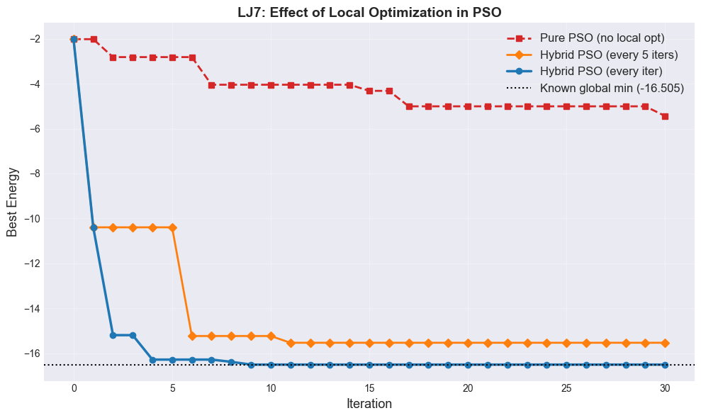
Pure PSO final:            -5.4373
Hybrid PSO (every 5) final: -15.5331
Hybrid PSO (every 1) final: -16.5054
Known global min:           -16.505384

def pso_2d_visual(func, iters=50, pop_size=20, w=0.7, c1=1.5, c2=1.5,
                  x_range=(-5, 5), y_range=(-5, 5)):
    """PSO on 2D function, tracking all positions for animation.
    
    Returns:
    --------
    X_history : list of (pop_size, 2) arrays
        Particle positions at each iteration
    scores_history : list of (pop_size,) arrays
        Fitness at each iteration
    g_best_hist : list
        Global best score at each iteration
    """
    X = np.random.uniform(x_range[0], x_range[1], size=(pop_size, 2))
    V = (np.random.random((pop_size, 2)) - 0.5) * 0.5
    
    scores = np.array([func(x) for x in X])
    p_best_X = X.copy()
    p_best_score = scores.copy()
    g_idx = np.argmin(scores)
    g_best_X = X[g_idx].copy()
    g_best_score = scores[g_idx]
    
    X_history = [X.copy()]
    scores_history = [scores.copy()]
    g_best_hist = [g_best_score]
    
    for iteration in range(iters):
        for i in range(pop_size):
            if scores[i] < p_best_score[i]:
                p_best_score[i] = scores[i]
                p_best_X[i] = X[i].copy()
        
        idx = np.argmin(p_best_score)
        if p_best_score[idx] < g_best_score:
            g_best_score = p_best_score[idx]
            g_best_X = p_best_X[idx].copy()
        
        r1 = np.random.random((pop_size, 2))
        r2 = np.random.random((pop_size, 2))
        V = (w*V + c1*r1*(p_best_X - X) + c2*r2*(g_best_X - X))
        X = X + V
        X = np.clip(X, x_range[0], x_range[1])
        
        scores = np.array([func(x) for x in X])
        
        X_history.append(X.copy())
        scores_history.append(scores.copy())
        g_best_hist.append(g_best_score)
    
    return X_history, scores_history, g_best_hist

print('Running PSO on 2D Ackley function...')
X_hist_ack, scores_hist_ack, g_best_ack = pso_2d_visual(
    ackley_2d, iters=50, pop_size=15, w=0.7, c1=1.5, c2=1.5,
    x_range=(-5, 5), y_range=(-5, 5)
)
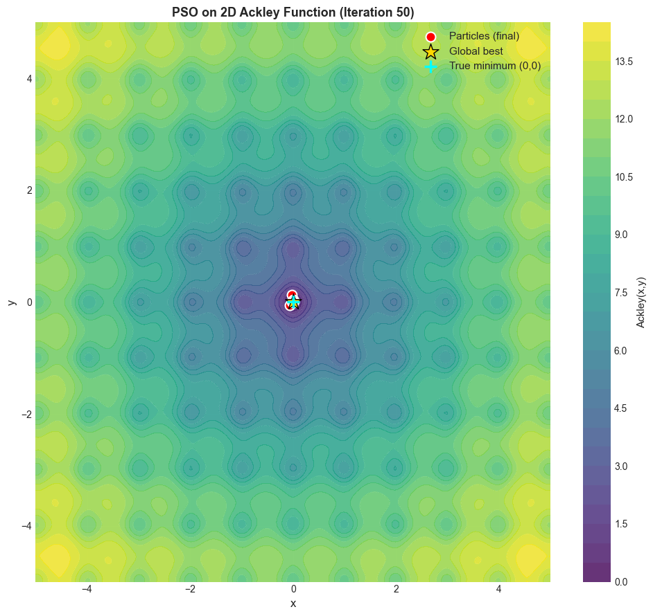
print(f'Converged to f(x,y) = {g_best_ack[-1]:.4f}')
print(f'Expected minimum: f(0,0) = 0.0')

Running PSO on 2D Ackley function...
Converged to f(x,y) = 0.0003
Expected minimum: f(0,0) = 0.0

# Create contour plot with final particle positions
fig, ax = plt.subplots(figsize=(10, 9))

x = np.linspace(-5, 5, 200)
y = np.linspace(-5, 5, 200)
X_grid, Y_grid = np.meshgrid(x, y)
Z = np.zeros_like(X_grid)
for i in range(len(x)):
    for j in range(len(y)):
        Z[j, i] = ackley_2d([X_grid[j, i], Y_grid[j, i]])

contour = ax.contourf(X_grid, Y_grid, Z, levels=30, cmap='viridis', alpha=0.8)
ax.contour(X_grid, Y_grid, Z, levels=10, colors='white', linewidths=0.5, alpha=0.3)
cbar = plt.colorbar(contour, ax=ax)
cbar.set_label('Ackley(x,y)', fontsize=11)

# Plot final particle positions
X_final = X_hist_ack[-1]
ax.scatter(X_final[:, 0], X_final[:, 1], c='red', s=100, 
          marker='o', edgecolors='white', linewidth=1.5, label='Particles (final)', zorder=5)

# Mark global best
g_best_idx = np.argmin(scores_hist_ack[-1])
ax.scatter(X_final[g_best_idx, 0], X_final[g_best_idx, 1], 
          c='gold', s=300, marker='*', edgecolors='black', linewidth=1, 
          label='Global best', zorder=6)

# Mark true minimum
ax.scatter(0, 0, c='cyan', s=150, marker='+', linewidth=2.5, 
          label='True minimum (0,0)', zorder=6)

ax.set_xlabel('x', fontsize=12)
ax.set_ylabel('y', fontsize=12)
ax.set_title('PSO on 2D Ackley Function (Iteration 50)', fontsize=13, fontweight='bold')
ax.legend(fontsize=11, loc='upper right')
ax.grid(True, alpha=0.2)
plt.tight_layout()
plt.show()

from matplotlib.animation import FuncAnimation
from IPython.display import HTML

# Create animation of PSO on Ackley
fig, ax = plt.subplots(figsize=(10, 9))

# Background contours
x = np.linspace(-5, 5, 150)
y = np.linspace(-5, 5, 150)
X_grid, Y_grid = np.meshgrid(x, y)
Z = np.zeros_like(X_grid)
for i in range(len(x)):
    for j in range(len(y)):
        Z[j, i] = ackley_2d([X_grid[j, i], Y_grid[j, i]])

contour = ax.contourf(X_grid, Y_grid, Z, levels=25, cmap='viridis', alpha=0.8)
ax.contour(X_grid, Y_grid, Z, levels=8, colors='white', linewidths=0.4, alpha=0.3)
plt.colorbar(contour, ax=ax, label='f(x,y)')

# True minimum
ax.scatter(0, 0, c='cyan', s=150, marker='+', linewidth=2.5, 
          label='True min (0,0)', zorder=6)

# Initialize particle scatter
scat = ax.scatter([], [], c='red', s=80, marker='o', edgecolors='white', 
                 linewidth=1.5, label='Particles', zorder=5)
best_point, = ax.plot([], [], 'g*', markersize=20, label='Current best', zorder=6)

title = ax.set_title('')
ax.set_xlim(-5, 5)
ax.set_ylim(-5, 5)
ax.set_xlabel('x', fontsize=11)
ax.set_ylabel('y', fontsize=11)
ax.legend(fontsize=10, loc='upper right')
ax.grid(True, alpha=0.2)

def update(frame):
    if frame < len(X_hist_ack):
        X_frame = X_hist_ack[frame]
        scat.set_offsets(X_frame)
        
        # Find and mark best in this frame
        scores_frame = scores_hist_ack[frame]
        best_idx = np.argmin(scores_frame)
        best_point.set_data([X_frame[best_idx, 0]], [X_frame[best_idx, 1]])
        
        title.set_text(f'PSO on 2D Ackley | Iter {frame} | Best f = {g_best_ack[frame]:.4f}')
    return scat, best_point, title

ani = FuncAnimation(fig, update, frames=len(X_hist_ack), 
                   interval=200, blit=True, repeat=True)
plt.tight_layout()
HTML(ani.to_jshtml())

Once Loop Reflect