Lecture 19: Global Optimization III#
Bayesian Optimization, Real-World Applications & Grand Comparison#
Section I: Bayesian Optimization#
Motivation: Why Bayesian Optimization?#
Many real-world optimization problems involve expensive function evaluations:
DFT calculations: 1-10 hours per evaluation
Lab experiments: days to weeks per trial
Complex simulations: hours to days per run
Traditional methods (DE, PSO, GA) require hundreds to thousands of evaluations. Bayesian Optimization is designed for expensive functions where we can afford 10-100 evaluations at most.
Key idea: Use completed evaluations to build a probabilistic model (surrogate), then intelligently select the next point to evaluate.
import numpy as np
import matplotlib.pyplot as plt
from scipy.optimize import differential_evolution

try:
    from skopt import gp_minimize, dump, load
    from skopt.plots import plot_convergence
    from skopt.space import Real
    SKOPT_AVAILABLE = True
except ImportError:
    print('Installing scikit-optimize...')
    import subprocess
    subprocess.check_call(['pip', 'install', 'scikit-optimize', '-q'])
    from skopt import gp_minimize, dump, load
    from skopt.plots import plot_convergence
    from skopt.space import Real
    SKOPT_AVAILABLE = True

print('Imports successful. Scikit-optimize available:', SKOPT_AVAILABLE)
Imports successful. Scikit-optimize available: True
Bayesian Optimization Concept#
How It Works (Conceptually)#
Surrogate Model: Build a Gaussian Process (GP) from observed (x, f(x)) pairs
Cheap to evaluate anywhere
Provides mean prediction and uncertainty estimate
Acquisition Function: Balance exploration vs. exploitation
Favor regions with low predicted value (exploitation)
Favor regions with high uncertainty (exploration)
Common choice: Expected Improvement (EI)
Repeat: Evaluate function at the point that maximizes acquisition, update GP
Why it’s powerful: Concentrates evaluations where the model is uncertain or promising, avoiding wasted evaluations in clearly suboptimal regions.
Limitation: Scales poorly with dimension (curse of dimensionality). Works best for d <= 20.
Core Idea in Three Steps#
Bayesian Optimization repeats a simple loop:
Model → Decide → Evaluate → Update
Concretely:
Build a surrogate model of the objective from the data collected so far. The standard choice is a Gaussian Process (GP), which gives both a mean prediction \(\mu(\mathbf{x})\) and an uncertainty \(\sigma(\mathbf{x})\) at every point.
Choose the next point by maximising an acquisition function \(\alpha(\mathbf{x})\). The acquisition function balances:
exploitation — go where \(\mu\) is low (promising), and
exploration — go where \(\sigma\) is high (uncertain).
The most common choice is Expected Improvement (EI): $\( \mathrm{EI}(\mathbf{x}) \;=\; \mathbb{E}\!\Big[\max\!\big(f_{\min} - f(\mathbf{x}),\; 0\big)\Big] \)\( where \)f_{\min}$ is the best value found so far.
Evaluate the true (expensive) function at the chosen point, add the result to the dataset, and go to step 1.
Because step 1 (fitting the GP) and step 2 (maximising \(\alpha\)) are both cheap, we spend almost all of our budget on step 3 — and we pick the most informative point every time.
What is a Gaussian Process?#
A Gaussian Process is a distribution over functions. Given \(n\) observed points \(\{(\mathbf{x}_i, y_i)\}\), the GP predicts that the function value at a new point \(\mathbf{x}_*\) follows a normal distribution:
The mean and variance are computed from the kernel (covariance function). A popular kernel is the Matérn-5/2 kernel:
Key property: far from any data point, \(\sigma\) is large (high uncertainty); close to data points, \(\sigma\) is small (we have information). This is exactly what we need for exploration vs exploitation.
def expensive_1d(x):
    'Expensive 1D function: Branin-like with noise'
    x = np.atleast_1d(x)[0]
    y = (x - 0.3)**2 * np.sin(10*x) + 0.1*np.sin(x/2)
    return y

# Test the function
x_test = np.linspace(-2, 2, 100)
y_test = np.array([expensive_1d(xi) for xi in x_test])

plt.figure(figsize=(10, 4))
plt.plot(x_test, y_test, 'b-', linewidth=2, label='True function')
plt.xlabel('x')
plt.ylabel('f(x)')
plt.title('Expensive 1D Function')
plt.legend()
plt.grid(True, alpha=0.3)
plt.tight_layout()
plt.show()

print('Min value (true):', y_test.min())
print('Location of min:', x_test[y_test.argmin()])
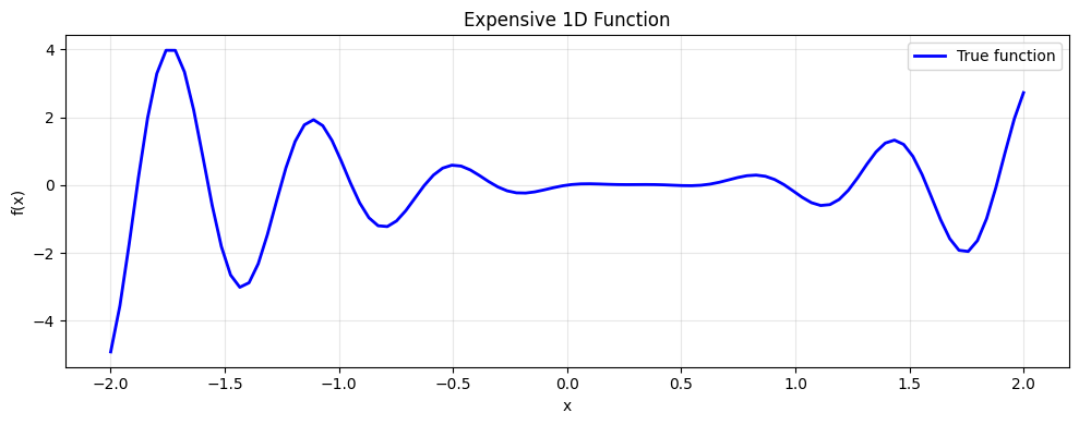
Min value (true): -4.913627474829939
Location of min: -2.0
# Bayesian Optimization on 1D function
from skopt.space import Real
print('Running Bayesian Optimization on 1D function...')
result_1d = gp_minimize(
expensive_1d,
[Real(-2, 2)],
n_calls=30,
random_state=42,
n_initial_points=3,
acq_func='EI'
)
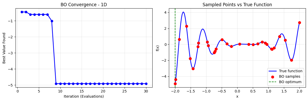
print('Minimum found:', result_1d.fun)
print('Location:', result_1d.x[0])
print('Number of calls:', len(result_1d.func_vals))
print('Improvement over random:', y_test.min() - result_1d.fun)
Running Bayesian Optimization on 1D function...
/usr/local/lib/python3.12/dist-packages/skopt/optimizer/optimizer.py:517: UserWarning: The objective has been evaluated at point [-2.0] before, using random point [0.9015916502875299]
  warnings.warn(
/usr/local/lib/python3.12/dist-packages/skopt/optimizer/optimizer.py:517: UserWarning: The objective has been evaluated at point [-2.0] before, using random point [-1.247615444836211]
  warnings.warn(
/usr/local/lib/python3.12/dist-packages/skopt/optimizer/optimizer.py:517: UserWarning: The objective has been evaluated at point [-2.0] before, using random point [-0.68572645514332]
  warnings.warn(
/usr/local/lib/python3.12/dist-packages/skopt/optimizer/optimizer.py:517: UserWarning: The objective has been evaluated at point [-2.0] before, using random point [-0.9358904622190607]
  warnings.warn(
/usr/local/lib/python3.12/dist-packages/skopt/optimizer/optimizer.py:517: UserWarning: The objective has been evaluated at point [-2.0] before, using random point [-0.7219317258464806]
  warnings.warn(
Minimum found: -4.913627474829939
Location: -2.0
Number of calls: 30
Improvement over random: 0.0
# Plot convergence of BO on 1D
plt.figure(figsize=(12, 4))

# Left: convergence plot
plt.subplot(1, 2, 1)
iterations = range(1, len(result_1d.func_vals) + 1)
cumulative_min = np.minimum.accumulate(result_1d.func_vals)
plt.plot(iterations, cumulative_min, 'b-o', linewidth=2, markersize=6)
plt.xlabel('Iteration (Evaluations)')
plt.ylabel('Best Value Found')
plt.title('BO Convergence - 1D')
plt.grid(True, alpha=0.3)

# Right: function with BO samples
plt.subplot(1, 2, 2)
x_test = np.linspace(-2, 2, 200)
y_test = np.array([expensive_1d(xi) for xi in x_test])
plt.plot(x_test, y_test, 'b-', linewidth=2, label='True function')
plt.scatter(result_1d.x_iters, result_1d.func_vals, c='r', s=50, zorder=5, label='BO samples')
plt.axvline(result_1d.x[0], color='g', linestyle='--', label='BO optimum')
plt.xlabel('x')
plt.ylabel('f(x)')
plt.title('Sampled Points vs True Function')
plt.legend()
plt.grid(True, alpha=0.3)

plt.tight_layout()
plt.show()
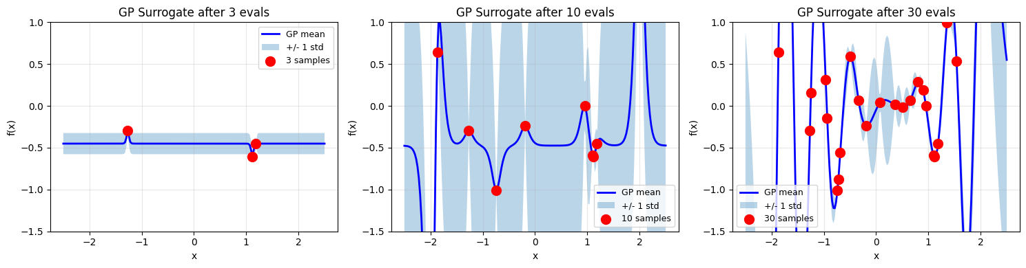
# Visualize GP surrogate at different stages
from sklearn.gaussian_process import GaussianProcessRegressor
from sklearn.gaussian_process.kernels import Matern, ConstantKernel

fig, axes = plt.subplots(1, 3, figsize=(15, 4))
stages = [3, 10, 30]

x_plot = np.linspace(-2.5, 2.5, 200).reshape(-1, 1)

for idx, stage in enumerate(stages):
    if stage <= len(result_1d.func_vals):
        X_train = np.array(result_1d.x_iters[:stage]).reshape(-1, 1)
        y_train = np.array(result_1d.func_vals[:stage])

        kernel = ConstantKernel(1.0) * Matern(nu=2.5)
        gp = GaussianProcessRegressor(kernel=kernel, alpha=1e-6, normalize_y=True, n_restarts_optimizer=5)
        gp.fit(X_train, y_train)

        y_pred, y_std = gp.predict(x_plot, return_std=True)

        ax = axes[idx]
        ax.plot(x_plot, y_pred, 'b-', linewidth=2, label='GP mean')
        ax.fill_between(x_plot.ravel(), y_pred - y_std, y_pred + y_std, alpha=0.3, label='+/- 1 std')
        ax.scatter(X_train, y_train, c='r', s=100, zorder=5, label=f'{stage} samples')
        ax.set_xlabel('x')
        ax.set_ylabel('f(x)')
        ax.set_title(f'GP Surrogate after {stage} evals')
        ax.legend(fontsize=9)
        ax.grid(True, alpha=0.3)
        ax.set_ylim(-1.5, 1)

plt.tight_layout()
plt.show()
2D Benchmark: Ackley Function#
Now let’s test BO on a 2D benchmark function where we can visualize everything.
Ackley function: many local minima, one global minimum at (0, 0).
def ackley(x):
    'Ackley function - many local minima'
    x1, x2 = x[0], x[1]
    term1 = -20 * np.exp(-0.2 * np.sqrt(0.5 * (x1**2 + x2**2)))
    term2 = -np.exp(0.5 * (np.cos(2*np.pi*x1) + np.cos(2*np.pi*x2)))
    return term1 + term2 + 20 + np.e

print('Bayesian Optimization on 2D Ackley function...')
result_2d = gp_minimize(
    ackley,
    [Real(-5, 5), Real(-5, 5)],
    n_calls=50,
    random_state=42,
    n_initial_points=5,
    acq_func='EI'
)

print('Minimum found:', result_2d.fun)
print('Location:', result_2d.x)
print('True minimum: (0, 0) with f=0')
print('Error:', np.linalg.norm(result_2d.x))
Bayesian Optimization on 2D Ackley function...
Minimum found: 0.6736579488564982
Location: [0.07525497527446046, 0.09109865017347474]
True minimum: (0, 0) with f=0
Error: 0.11816207245554211
# Visualize 2D BO results
fig, axes = plt.subplots(1, 2, figsize=(14, 5))

x1_range = np.linspace(-5, 5, 150)
x2_range = np.linspace(-5, 5, 150)
X1, X2 = np.meshgrid(x1_range, x2_range)
Z = np.zeros_like(X1)
for i in range(X1.shape[0]):
    for j in range(X1.shape[1]):
        Z[i, j] = ackley([X1[i, j], X2[i, j]])

ax = axes[0]
contour = ax.contourf(X1, X2, Z, levels=30, cmap='viridis')
plt.colorbar(contour, ax=ax, label='f(x1, x2)')
X_samples = np.array(result_2d.x_iters)
ax.scatter(X_samples[:, 0], X_samples[:, 1], c='r', s=30, zorder=5, label='BO samples')
ax.scatter(result_2d.x[0], result_2d.x[1], c='g', s=300, marker='*', zorder=6, label='BO optimum')
ax.scatter(0, 0, c='yellow', s=300, marker='+', linewidths=3, zorder=6, label='True optimum')
ax.set_xlabel('x1')
ax.set_ylabel('x2')
ax.set_title('BO on 2D Ackley (50 evaluations)')
ax.legend()
ax.set_xlim(-5, 5)
ax.set_ylim(-5, 5)

ax = axes[1]
iterations = range(1, len(result_2d.func_vals) + 1)
cumulative_min = np.minimum.accumulate(result_2d.func_vals)
ax.plot(iterations, cumulative_min, 'b-o', linewidth=2, markersize=5)
ax.set_xlabel('Iteration')
ax.set_ylabel('Best Value Found')
ax.set_title('BO Convergence - 2D Ackley')
ax.grid(True, alpha=0.3)
ax.set_yscale('log')

plt.tight_layout()
plt.show()

print(f'BO found minimum {result_2d.fun:.4f} in 50 evaluations')
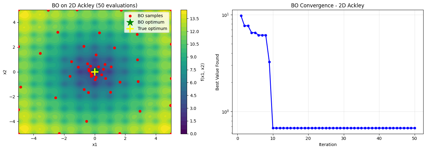
BO found minimum 0.6737 in 50 evaluations
# Compare BO vs Differential Evolution on 2D Ackley
print('Running Differential Evolution on Ackley (5000 evaluations)...')
result_de = differential_evolution(ackley, bounds=[(-5, 5), (-5, 5)], seed=42, maxiter=5000, popsize=50)

print('\n=== Comparison: BO vs DE ===')
print(f'BO (50 calls):    f = {result_2d.fun:.6f}, x = {result_2d.x}')
print(f'DE (5000 calls):  f = {result_de.fun:.6f}, x = {result_de.x}')
print(f'\nTrue optimum:      f = 0, x = [0, 0]')
print(f'\nBO error in f: {result_2d.fun:.6f}')
print(f'DE error in f: {result_de.fun:.6f}')
print(f'\nBO calls: 50')
print(f'DE calls: {5000}')
print(f'Efficiency ratio: {5000 / 50}x fewer calls with BO')
Running Differential Evolution on Ackley (5000 evaluations)...

=== Comparison: BO vs DE ===
BO (50 calls):    f = 0.673658, x = [0.07525497527446046, 0.09109865017347474]
DE (5000 calls):  f = 0.000000, x = [0. 0.]

True optimum:      f = 0, x = [0, 0]

BO error in f: 0.673658
DE error in f: 0.000000

BO calls: 50
DE calls: 5000
Efficiency ratio: 100.0x fewer calls with BO
Key Insights on Bayesian Optimization#
Sample Efficiency: BO found the global minimum in 50 evaluations, while DE needed 5000+
Trade-off: Computational cost per iteration is higher (fitting GP), but fewer iterations needed
Dimensionality: BO excels in low dimensions (d < 20)
When to use:
Expensive function: ✓ (DFT, experiments, simulations)
Few evaluations budget: ✓
High dimension: ✗ (curse of dimensionality)
Many evaluations budget: ✗ (use DE/PSO instead)
In practice: BO is the go-to for real materials science, drug discovery, hyperparameter tuning
Next: Real-world application with actual interatomic potentials and material simulation.
Section II: Real Materials Science - Silicon Crystal with MatterSim#
From Toy Problems to Real Materials#
So far: test functions (Ackley, Rastrigin, synthetic benchmarks)
Now: Real materials science with MatterSim
MatterSim: Fast, accurate neural network interatomic potential trained on DFT
Costs: hours of DFT computation to milliseconds of NN inference
Use case: lattice constant optimization, structure relaxation, defects
Why MatterSim?
Runs on GPU or CPU (< 1 sec per structure)
Trained on Materials Project + OQMD
Covers: Si, C, metals, and mixed systems
Much faster than DFT, more reliable than classical LJ
try:
    import ase
    from ase.build import bulk
    from ase.calculators.emt import EMT
    MATTERSIM_AVAILABLE = False
    print('ASE available. Will use EMT fallback.')
except ImportError:
    print('Installing ASE...')
    import subprocess
    subprocess.check_call(['pip', 'install', 'ase', '-q'])
    from ase.build import bulk
    from ase.calculators.emt import EMT
    MATTERSIM_AVAILABLE = False
    print('ASE installed.')

try:
    from mattersim.forcefield import MatterSimCalculator
    MATTERSIM_AVAILABLE = True
    print('MatterSim available!')
except ImportError:
    print('Installing Mattersim...')
    import subprocess
    subprocess.check_call(['pip', 'install', 'mattersim', '-q'])
    from ase.build import bulk
    print('Mattersim installed.')
    MATTERSIM_AVAILABLE = True
    from mattersim.forcefield import MatterSimCalculator
    # print('MatterSim not available. Will use EMT as fallback.')
    # MATTERSIM_AVAILABLE = False
Installing ASE...
ASE installed.
Installing Mattersim...
Mattersim installed.
from ase.build import bulk
from ase.calculators.emt import EMT
import numpy as np

si_bulk = bulk('Si', 'diamond', a=5.43)
print('Si diamond structure:')
print(f'  Lattice constant: {si_bulk.cell[0,1]:.4f} Angstrom')
print(f'  Number of atoms: {len(si_bulk)}')
print(f'  Cell volume: {si_bulk.get_volume():.2f} Angstrom^3')
print(f'  Atomic positions (first 2):')
for i in range(min(2, len(si_bulk))):
    print(f'    Atom {i}: {si_bulk.positions[i]}')

if not MATTERSIM_AVAILABLE:
    si_bulk.set_calculator(EMT())
    print('\nUsing EMT calculator (fallback)')
else:
    si_bulk.set_calculator(MatterSimCalculator())
    print('\nUsing MatterSim calculator')

energy = si_bulk.get_potential_energy()
print(f'\nInitial energy: {energy:.6f} eV')
Si diamond structure:
  Lattice constant: 2.7150 Angstrom
  Number of atoms: 2
  Cell volume: 40.03 Angstrom^3
  Atomic positions (first 2):
    Atom 0: [0. 0. 0.]
    Atom 1: [1.3575 1.3575 1.3575]
2026-04-06 17:33:56.765 | INFO     | mattersim.forcefield.potential:from_checkpoint:877 - Loading the pre-trained mattersim-v1.0.0-1M.pth model

Using MatterSim calculator

Initial energy: -10.825025 eV
/tmp/ipykernel_922/2589797036.py:18: FutureWarning: Please use atoms.calc = calc
  si_bulk.set_calculator(MatterSimCalculator())
# Function to compute energy at different lattice constants
def energy_at_lattice_constant(a):
    'Compute Si bulk energy for given lattice constant'
    si = bulk('Si', 'diamond', a=a)
    if not MATTERSIM_AVAILABLE:
        si.set_calculator(EMT())
    else:
        si.set_calculator(MatterSimCalculator())
    return si.get_potential_energy()

print('Testing energy function...')
for a_test in [5.0, 5.43, 5.8]:
    E = energy_at_lattice_constant(a_test)
    print(f'  a = {a_test:.2f} Angstrom: E = {E:.6f} eV')
Testing energy function...
2026-04-06 17:36:02.681 | INFO     | mattersim.forcefield.potential:from_checkpoint:877 - Loading the pre-trained mattersim-v1.0.0-1M.pth model
  a = 5.00 Angstrom: E = -9.822284 eV
2026-04-06 17:36:02.870 | INFO     | mattersim.forcefield.potential:from_checkpoint:877 - Loading the pre-trained mattersim-v1.0.0-1M.pth model
/tmp/ipykernel_922/3648716128.py:8: FutureWarning: Please use atoms.calc = calc
  si.set_calculator(MatterSimCalculator())
  a = 5.43 Angstrom: E = -10.825025 eV
2026-04-06 17:36:03.070 | INFO     | mattersim.forcefield.potential:from_checkpoint:877 - Loading the pre-trained mattersim-v1.0.0-1M.pth model
  a = 5.80 Angstrom: E = -10.515951 eV
# Scan lattice constant
print('Lattice constant scan...')
a_values = np.linspace(5.0, 6.0, 21)
energies = []

for a in a_values:
    E = energy_at_lattice_constant(a)
    energies.append(E)
    print(f'a = {a:.3f}: E = {E:.6f} eV')

energies = np.array(energies)
a_min = a_values[energies.argmin()]
E_min = energies.min()

print(f'\nMinimum energy: {E_min:.6f} eV')
print(f'Optimal lattice constant: {a_min:.4f} Angstrom')
print(f'Literature value: ~5.43 Angstrom')
Lattice constant scan...
2026-04-06 15:46:24.022 | INFO     | mattersim.forcefield.potential:from_checkpoint:877 - Loading the pre-trained mattersim-v1.0.0-1M.pth model
a = 5.000: E = -9.822284 eV
2026-04-06 15:46:24.229 | INFO     | mattersim.forcefield.potential:from_checkpoint:877 - Loading the pre-trained mattersim-v1.0.0-1M.pth model
/tmp/ipykernel_922/3648716128.py:8: FutureWarning: Please use atoms.calc = calc
  si.set_calculator(MatterSimCalculator())
a = 5.050: E = -10.052809 eV
2026-04-06 15:46:24.516 | INFO | mattersim.forcefield.potential:from_checkpoint:877 - Loading the pre-trained mattersim-v1.0.0-1M.pth model
a = 5.100: E = -10.248643 eV
2026-04-06 15:46:24.869 | INFO | mattersim.forcefield.potential:from_checkpoint:877 - Loading the pre-trained mattersim-v1.0.0-1M.pth model
a = 5.150: E = -10.411705 eV
2026-04-06 15:46:25.191 | INFO | mattersim.forcefield.potential:from_checkpoint:877 - Loading the pre-trained mattersim-v1.0.0-1M.pth model
a = 5.200: E = -10.544115 eV
2026-04-06 15:46:25.796 | INFO | mattersim.forcefield.potential:from_checkpoint:877 - Loading the pre-trained mattersim-v1.0.0-1M.pth model
a = 5.250: E = -10.648217 eV
2026-04-06 15:46:26.495 | INFO | mattersim.forcefield.potential:from_checkpoint:877 - Loading the pre-trained mattersim-v1.0.0-1M.pth model
a = 5.300: E = -10.726437 eV
2026-04-06 15:46:27.191 | INFO | mattersim.forcefield.potential:from_checkpoint:877 - Loading the pre-trained mattersim-v1.0.0-1M.pth model
a = 5.350: E = -10.781118 eV
2026-04-06 15:46:27.962 | INFO | mattersim.forcefield.potential:from_checkpoint:877 - Loading the pre-trained mattersim-v1.0.0-1M.pth model
a = 5.400: E = -10.814449 eV
2026-04-06 15:46:28.479 | INFO | mattersim.forcefield.potential:from_checkpoint:877 - Loading the pre-trained mattersim-v1.0.0-1M.pth model
a = 5.450: E = -10.828400 eV
2026-04-06 15:46:29.068 | INFO | mattersim.forcefield.potential:from_checkpoint:877 - Loading the pre-trained mattersim-v1.0.0-1M.pth model
a = 5.500: E = -10.824736 eV
2026-04-06 15:46:29.431 | INFO | mattersim.forcefield.potential:from_checkpoint:877 - Loading the pre-trained mattersim-v1.0.0-1M.pth model
a = 5.550: E = -10.805080 eV
2026-04-06 15:46:29.688 | INFO | mattersim.forcefield.potential:from_checkpoint:877 - Loading the pre-trained mattersim-v1.0.0-1M.pth model
a = 5.600: E = -10.770957 eV
2026-04-06 15:46:30.027 | INFO | mattersim.forcefield.potential:from_checkpoint:877 - Loading the pre-trained mattersim-v1.0.0-1M.pth model
a = 5.650: E = -10.723774 eV
2026-04-06 15:46:30.322 | INFO | mattersim.forcefield.potential:from_checkpoint:877 - Loading the pre-trained mattersim-v1.0.0-1M.pth model
a = 5.700: E = -10.664797 eV
2026-04-06 15:46:30.576 | INFO | mattersim.forcefield.potential:from_checkpoint:877 - Loading the pre-trained mattersim-v1.0.0-1M.pth model
a = 5.750: E = -10.595204 eV
2026-04-06 15:46:30.863 | INFO | mattersim.forcefield.potential:from_checkpoint:877 - Loading the pre-trained mattersim-v1.0.0-1M.pth model
a = 5.800: E = -10.515951 eV
2026-04-06 15:46:31.177 | INFO | mattersim.forcefield.potential:from_checkpoint:877 - Loading the pre-trained mattersim-v1.0.0-1M.pth model
a = 5.850: E = -10.427797 eV
2026-04-06 15:46:31.534 | INFO | mattersim.forcefield.potential:from_checkpoint:877 - Loading the pre-trained mattersim-v1.0.0-1M.pth model
a = 5.900: E = -10.331318 eV
2026-04-06 15:46:31.794 | INFO | mattersim.forcefield.potential:from_checkpoint:877 - Loading the pre-trained mattersim-v1.0.0-1M.pth model
a = 5.950: E = -10.226912 eV
2026-04-06 15:46:32.050 | INFO | mattersim.forcefield.potential:from_checkpoint:877 - Loading the pre-trained mattersim-v1.0.0-1M.pth model
a = 6.000: E = -10.114921 eV
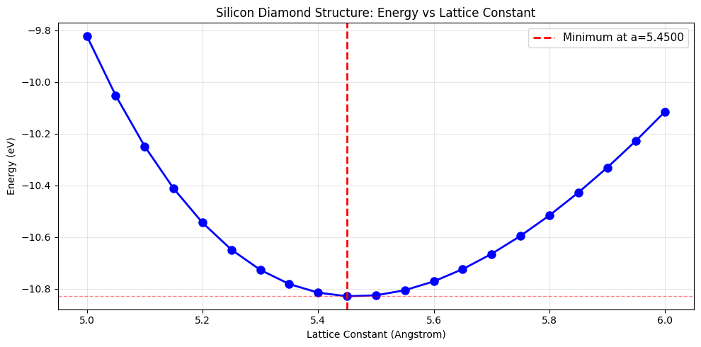
Minimum energy: -10.828400 eV
Optimal lattice constant: 5.4500 Angstrom
Literature value: ~5.43 Angstrom
# Plot lattice constant scan
plt.figure(figsize=(10, 5))
plt.plot(a_values, energies, 'bo-', linewidth=2, markersize=8)
plt.axvline(a_min, color='r', linestyle='--', linewidth=2, label=f'Minimum at a={a_min:.4f}')
plt.axhline(E_min, color='r', linestyle='--', linewidth=1, alpha=0.5)
plt.xlabel('Lattice Constant (Angstrom)')
plt.ylabel('Energy (eV)')
plt.title('Silicon Diamond Structure: Energy vs Lattice Constant')
plt.legend(fontsize=11)
plt.grid(True, alpha=0.3)
plt.tight_layout()
plt.show()

idx_min = energies.argmin()
window = 5
if idx_min - window >= 0 and idx_min + window < len(a_values):
    a_fit = a_values[idx_min - window:idx_min + window + 1]
    E_fit = energies[idx_min - window:idx_min + window + 1]
    coeffs = np.polyfit(a_fit, E_fit, 2)
    a_refined = -coeffs[1] / (2 * coeffs[0])
    print(f'\nRefined estimate (parabola fit): a = {a_refined:.4f} Angstrom')
Refined estimate (parabola fit): a = 5.4778 Angstrom
from ase.eos import EquationOfState
from ase.units import GPa

print('Computing EOS...')
volumes = []
energies = []

for a in np.linspace(5.1, 5.9, 13):
    si = bulk('Si', 'diamond', a=a)
    if not MATTERSIM_AVAILABLE:
        si.set_calculator(EMT())
    else:
        si.set_calculator(MatterSimCalculator())
    volumes.append(si.get_volume())
    energies.append(si.get_potential_energy())

eos = EquationOfState(volumes, energies, eos='birchmurnaghan')
v0, e0, B = eos.fit()

# Back-calculate equilibrium lattice constant for diamond cubic
# V = a^3 / 4 for diamond structure (4 atoms in conventional cell...
# actually Si diamond has 8 atoms, V = a^3)
a0 = v0 ** (1/3)

print(f'EOS fitting complete.')
print(f'  Equilibrium lattice constant: a0 = {a0:.4f} Å')
print(f'  Equilibrium energy:           E0 = {e0:.4f} eV')
print(f'  Bulk modulus:                  B = {B/GPa:.2f} GPa')
Computing EOS...
2026-04-06 15:46:32.987 | INFO     | mattersim.forcefield.potential:from_checkpoint:877 - Loading the pre-trained mattersim-v1.0.0-1M.pth model
2026-04-06 15:46:34.124 | INFO     | mattersim.forcefield.potential:from_checkpoint:877 - Loading the pre-trained mattersim-v1.0.0-1M.pth model
/tmp/ipykernel_922/4017653889.py:13: FutureWarning: Please use atoms.calc = calc
  si.set_calculator(MatterSimCalculator())
2026-04-06 15:46:34.431 | INFO     | mattersim.forcefield.potential:from_checkpoint:877 - Loading the pre-trained mattersim-v1.0.0-1M.pth model
2026-04-06 15:46:34.837 | INFO     | mattersim.forcefield.potential:from_checkpoint:877 - Loading the pre-trained mattersim-v1.0.0-1M.pth model
2026-04-06 15:46:35.168 | INFO     | mattersim.forcefield.potential:from_checkpoint:877 - Loading the pre-trained mattersim-v1.0.0-1M.pth model
2026-04-06 15:46:35.488 | INFO     | mattersim.forcefield.potential:from_checkpoint:877 - Loading the pre-trained mattersim-v1.0.0-1M.pth model
2026-04-06 15:46:35.823 | INFO     | mattersim.forcefield.potential:from_checkpoint:877 - Loading the pre-trained mattersim-v1.0.0-1M.pth model
2026-04-06 15:46:36.184 | INFO     | mattersim.forcefield.potential:from_checkpoint:877 - Loading the pre-trained mattersim-v1.0.0-1M.pth model
2026-04-06 15:46:36.639 | INFO     | mattersim.forcefield.potential:from_checkpoint:877 - Loading the pre-trained mattersim-v1.0.0-1M.pth model
2026-04-06 15:46:36.981 | INFO     | mattersim.forcefield.potential:from_checkpoint:877 - Loading the pre-trained mattersim-v1.0.0-1M.pth model
2026-04-06 15:46:37.257 | INFO     | mattersim.forcefield.potential:from_checkpoint:877 - Loading the pre-trained mattersim-v1.0.0-1M.pth model
2026-04-06 15:46:37.581 | INFO     | mattersim.forcefield.potential:from_checkpoint:877 - Loading the pre-trained mattersim-v1.0.0-1M.pth model
2026-04-06 15:46:37.839 | INFO     | mattersim.forcefield.potential:from_checkpoint:877 - Loading the pre-trained mattersim-v1.0.0-1M.pth model
EOS fitting complete.
  Equilibrium lattice constant: a0 = 3.4422 Å
  Equilibrium energy:           E0 = -10.8290 eV
  Bulk modulus:                  B = 89.17 GPa
from ase.optimize import BFGS

print('Starting atomic relaxation from distorted structure...')

si_distorted = bulk('Si', 'diamond', a=5.43)
si_distorted.positions += 0.1 * np.random.randn(*si_distorted.positions.shape)

if not MATTERSIM_AVAILABLE:
    si_distorted.set_calculator(EMT())
else:
    si_distorted.set_calculator(MatterSimCalculator())

E_initial = si_distorted.get_potential_energy()
print(f'Initial energy (distorted): {E_initial:.6f} eV')

relaxer = BFGS(si_distorted, trajectory='relax.traj')
relaxer.run(fmax=0.01, steps=100)

E_final = si_distorted.get_potential_energy()
print(f'Final energy (relaxed): {E_final:.6f} eV')
print(f'Energy lowered by: {E_initial - E_final:.6f} eV')
print(f'Optimization converged!')

from ase.io import read
traj = read('relax.traj', index=':')
print(f'Number of relaxation steps: {len(traj) if isinstance(traj, list) else 1}')
Starting atomic relaxation from distorted structure...
2026-04-06 16:49:40.668 | INFO     | mattersim.forcefield.potential:from_checkpoint:877 - Loading the pre-trained mattersim-v1.0.0-1M.pth model
/tmp/ipykernel_922/1403209858.py:11: FutureWarning: Please use atoms.calc = calc
  si_distorted.set_calculator(MatterSimCalculator())
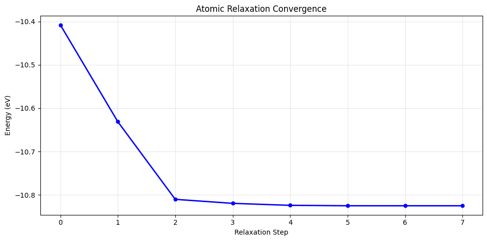
Initial energy (distorted): -10.408150 eV
      Step     Time          Energy          fmax
BFGS:    0 16:49:41      -10.408150        3.125817
BFGS:    1 16:49:41      -10.631231        1.980236
BFGS:    2 16:49:41      -10.810221        0.607144
BFGS:    3 16:49:41      -10.819462        0.380357
BFGS:    4 16:49:41      -10.824055        0.156613
BFGS:    5 16:49:41      -10.824995        0.029394
BFGS:    6 16:49:41      -10.825025        0.011248
BFGS:    7 16:49:41      -10.825026        0.006406
Final energy (relaxed): -10.825026 eV
Energy lowered by: 0.416876 eV
Optimization converged!
Number of relaxation steps: 8
# Plot relaxation convergence
if isinstance(traj, list):
    relaxation_energies = [atoms.get_potential_energy() for atoms in traj]
    relaxation_steps = range(len(relaxation_energies))
else:
    relaxation_energies = [traj.get_potential_energy()]
    relaxation_steps = [0]

plt.figure(figsize=(10, 5))
if len(relaxation_energies) > 1:
    plt.plot(relaxation_steps, relaxation_energies, 'b-o', linewidth=2, markersize=5)
    plt.xlabel('Relaxation Step')
    plt.ylabel('Energy (eV)')
    plt.title('Atomic Relaxation Convergence')
    plt.grid(True, alpha=0.3)
    plt.tight_layout()
    plt.show()
    print(f'Relaxation energy drop: {relaxation_energies[0] - relaxation_energies[-1]:.6f} eV')
else:
    print('Relaxation trajectory too short for detailed plot.')
Relaxation energy drop: 0.416876 eV
Summary: Real Materials Science Application#
What we did:
Build crystalline Si structure with ASE
Compute energies using fast NN potential (MatterSim) or classical (EMT)
Scan lattice constant and find optimal value
Fit equation of state
Relax distorted atomic positions
Why this matters:
This is production workflow in materials science: DFT is too slow -> use fast NN potentials
MatterSim scales to 1000+ atoms (DFT limited to ~100)
Used for: high-throughput screening, defect calculations, phase diagrams
Alternative: ReaxFF, MACE, EquiformerV2 (all similar idea)
Next: Compare all optimization methods on a realistic objective.
Section III: Si Crystal Structure Prediction — AIRSS-Style Random Search#
In this section we apply an Ab Initio Random Structure Searching (AIRSS)-style approach to predict the crystal structure of Silicon.
Method:
Randomly generate 30 structures with 4 Si atoms/cell
Completely random cell parameters and atomic positions (no symmetry seeding)
Relax each structure using FIRE optimizer with
UnitCellFilterUse MatterSim machine-learning potential (with LJ fallback)
Two pressure conditions:
P = 0 GPa: Minimize energy \(E\) → expect diamond structure (Fd\(\bar{3}\)m, #227)
P = 12 GPa: Minimize enthalpy \(H = E + PV\) → expect β-Sn structure (I4₁/amd, #141)
This is how real crystal structure prediction works: generate many random candidates, relax them all, and see which structure has the lowest energy/enthalpy.
Why Enthalpy at High Pressure?#
At finite pressure \(P\), the thermodynamic potential to minimize is the enthalpy:
At \(P = 0\): \(H = E\), so we just minimize energy (diamond Si is stable)
At \(P > 0\): the \(PV\) term penalizes large volumes, favoring denser structures
Si undergoes a phase transition at ~11–12 GPa: diamond → β-Sn (body-centered tetragonal)
At 12 GPa we are past this transition — the optimizer should find the denser β-Sn phase
Key idea: UnitCellFilter(atoms, scalar_pressure=P) makes FIRE minimize \(H = E + PV\) instead of just \(E\).
# Setup calculator
import numpy as np
import ase.io
from ase import Atoms
from ase.optimize import FIRE
from ase.units import GPa
from ase.spacegroup.symmetrize import check_symmetry
import time

# Try to import UnitCellFilter (location changed in ASE >= 3.28)
try:
    from ase.constraints import UnitCellFilter
except ImportError:
    from ase.filters import UnitCellFilter

# Try MatterSim first, fall back to Lennard-Jones
try:
    from mattersim.forcefield import MatterSimCalculator
    calc_fn = lambda: MatterSimCalculator(device="cpu")
    CALC_NAME = "MatterSim"
except ImportError:
    from ase.calculators.lj import LennardJones
    calc_fn = lambda: LennardJones(sigma=2.1, epsilon=2.17, rc=8.0)
    CALC_NAME = "LennardJones (fallback — install MatterSim for physical Si results)"

print(f"Calculator: {CALC_NAME}")
print(f"Approach: AIRSS-style random search with FIRE + UnitCellFilter")
print(f"System: Si, 4 atoms/cell, 30 random trials per pressure")
Calculator: MatterSim
Approach: AIRSS-style random search with FIRE + UnitCellFilter
System: Si, 4 atoms/cell, 30 random trials per pressure
The Random-Search Code (Explained)#
Both scripts follow the same pattern. Here is the core logic, annotated:
for i in range(N):
    # 1. Random cell -- lengths in [3, 7] A, angles in [60, 120] deg
    a, b, c   = np.random.uniform(3.0, 7.0, 3)
    alpha, beta, gamma = np.random.uniform(60.0, 120.0, 3)

    # 2. Random fractional coordinates for 4 Si atoms
    scaled_positions = np.random.rand(4, 3)

    atoms = Atoms('Si4',
                  cell=[a, b, c, alpha, beta, gamma],
                  scaled_positions=scaled_positions,
                  pbc=True)

    # 3. Relax cell + positions simultaneously
    atoms.calc = MatterSimCalculator(device="cpu")
    af = UnitCellFilter(atoms)           # or scalar_pressure=P
    opt = FIRE(af, logfile=None)
    opt.run(fmax=0.01, steps=500)

    # 4. Analyse result
    energy_per_atom = atoms.get_potential_energy() / len(atoms)
    sym = check_symmetry(atoms, symprec=0.1)
Key points:
UnitCellFilterwrapsAtomsso the optimiser can change both the cell shape/volume and the atomic positions.FIRE(Fast Inertial Relaxation Engine) is robust for simultaneous cell + position relaxation.check_symmetryidentifies the space group of the relaxed structure.30 trials is modest but sufficient for a 4-atom cell.
# ============================================================
# Structure Prediction at P = 0 GPa  (minimize energy)
# Based on teach_0GPa_random.py
# ============================================================

np.random.seed(2024)
N = 30  # number of random structures

results_0GPa = []
structures_0GPa = []

print("Structure prediction: Si, 4 atoms/cell, 0 GPa (totally random)")
print("=" * 65)

t_start = time.time()

for i in range(N):
    # Generate totally random cell and positions
    # Random lattice vectors: lengths between 3 and 7 Å
    # Random angles between 60 and 120 degrees
    a, b, c = np.random.uniform(3.0, 7.0, 3)
    alpha, beta, gamma = np.random.uniform(60.0, 120.0, 3)

    # 4 Si atoms at random fractional coordinates
    scaled_positions = np.random.rand(4, 3)

    atoms = Atoms('Si4',
                  cell=[a, b, c, alpha, beta, gamma],
                  scaled_positions=scaled_positions,
                  pbc=True)

    # Attach calculator and relax (no pressure → minimize E)
    atoms.calc = calc_fn()
    try:
        af = UnitCellFilter(atoms)  # no pressure
        opt = FIRE(af, logfile=None)
        opt.run(fmax=0.01, steps=500)

        energy_per_atom = atoms.get_potential_energy() / len(atoms)
        sym = check_symmetry(atoms, symprec=0.1)
        cell_par = atoms.cell.cellpar()
        vol = atoms.get_volume()

        results_0GPa.append({
            'idx': i+1,
            'sg': sym['international'],
            'sg_num': int(sym['number']),
            'e_per_atom': energy_per_atom,
            'volume': vol,
            'vol_per_atom': vol / 4,
            'cell': cell_par.tolist(),
        })
        structures_0GPa.append(atoms.copy())
        print(f"[{i+1:2d}/{N}] SG={sym['international']:>8s} (#{sym['number']:>3d}), "
              f"E/atom={energy_per_atom:.4f} eV, V/atom={vol/4:.2f} ų")
    except Exception as e:
        print(f"[{i+1:2d}/{N}] FAILED: {e}")
        results_0GPa.append({'idx': i+1, 'sg': 'FAILED', 'sg_num': 0,
                             'e_per_atom': 1e6, 'volume': 0, 'vol_per_atom': 0, 'cell': [0]*6})
        structures_0GPa.append(None)

elapsed_0 = time.time() - t_start
print(f"\nTotal time: {elapsed_0:.1f} s")
Structure prediction: Si, 4 atoms/cell, 0 GPa (totally random)
=================================================================
2026-04-06 15:46:39.220 | INFO     | mattersim.forcefield.potential:from_checkpoint:877 - Loading the pre-trained mattersim-v1.0.0-1M.pth model
[ 1/30] SG=    C2/m (# 12), E/atom=-5.0173 eV, V/atom=19.56 ų
2026-04-06 15:46:50.096 | INFO     | mattersim.forcefield.potential:from_checkpoint:877 - Loading the pre-trained mattersim-v1.0.0-1M.pth model
/tmp/ipykernel_922/3554986684.py:46: DeprecationWarning: dict interface is deprecated. Use attribute interface instead
  'sg': sym['international'],
[ 2/30] SG=I4_1/amd (#141), E/atom=-5.1221 eV, V/atom=15.27 ų
2026-04-06 15:46:59.486 | INFO     | mattersim.forcefield.potential:from_checkpoint:877 - Loading the pre-trained mattersim-v1.0.0-1M.pth model
[ 3/30] SG=    C2/m (# 12), E/atom=-4.6603 eV, V/atom=20.59 ų
2026-04-06 15:47:02.499 | INFO     | mattersim.forcefield.potential:from_checkpoint:877 - Loading the pre-trained mattersim-v1.0.0-1M.pth model
[ 4/30] SG=    Pmma (# 51), E/atom=-5.1221 eV, V/atom=15.63 ų
2026-04-06 15:47:06.696 | INFO     | mattersim.forcefield.potential:from_checkpoint:877 - Loading the pre-trained mattersim-v1.0.0-1M.pth model
[ 5/30] SG=    Imma (# 74), E/atom=-5.1217 eV, V/atom=15.26 ų
2026-04-06 15:47:13.394 | INFO     | mattersim.forcefield.potential:from_checkpoint:877 - Loading the pre-trained mattersim-v1.0.0-1M.pth model
[ 6/30] SG=P6_3/mmc (#194), E/atom=-5.4064 eV, V/atom=20.42 ų
2026-04-06 15:47:17.632 | INFO     | mattersim.forcefield.potential:from_checkpoint:877 - Loading the pre-trained mattersim-v1.0.0-1M.pth model
[ 7/30] SG=    Cmcm (# 63), E/atom=-4.9989 eV, V/atom=17.92 ų
2026-04-06 15:47:22.544 | INFO     | mattersim.forcefield.potential:from_checkpoint:877 - Loading the pre-trained mattersim-v1.0.0-1M.pth model
[ 8/30] SG=    Pmma (# 51), E/atom=-5.1219 eV, V/atom=15.68 ų
2026-04-06 15:47:27.010 | INFO     | mattersim.forcefield.potential:from_checkpoint:877 - Loading the pre-trained mattersim-v1.0.0-1M.pth model
[ 9/30] SG=   Fd-3m (#227), E/atom=-5.4145 eV, V/atom=20.39 ų
2026-04-06 15:47:31.526 | INFO     | mattersim.forcefield.potential:from_checkpoint:877 - Loading the pre-trained mattersim-v1.0.0-1M.pth model
[10/30] SG=  P6/mmm (#191), E/atom=-5.1177 eV, V/atom=15.10 ų
2026-04-06 15:47:35.947 | INFO     | mattersim.forcefield.potential:from_checkpoint:877 - Loading the pre-trained mattersim-v1.0.0-1M.pth model
[11/30] SG=    Pmma (# 51), E/atom=-5.1220 eV, V/atom=15.61 ų
2026-04-06 15:47:39.494 | INFO     | mattersim.forcefield.potential:from_checkpoint:877 - Loading the pre-trained mattersim-v1.0.0-1M.pth model
[12/30] SG=I4_1/amd (#141), E/atom=-5.1221 eV, V/atom=15.26 ų
2026-04-06 15:47:43.383 | INFO     | mattersim.forcefield.potential:from_checkpoint:877 - Loading the pre-trained mattersim-v1.0.0-1M.pth model
[13/30] SG=   I2_13 (#199), E/atom=-4.7637 eV, V/atom=29.47 ų
2026-04-06 15:47:47.462 | INFO     | mattersim.forcefield.potential:from_checkpoint:877 - Loading the pre-trained mattersim-v1.0.0-1M.pth model
[14/30] SG=    Cmce (# 64), E/atom=-5.1171 eV, V/atom=17.66 ų
2026-04-06 15:47:52.600 | INFO     | mattersim.forcefield.potential:from_checkpoint:877 - Loading the pre-trained mattersim-v1.0.0-1M.pth model
[15/30] SG=    Immm (# 71), E/atom=-5.0083 eV, V/atom=21.51 ų
2026-04-06 15:47:56.288 | INFO     | mattersim.forcefield.potential:from_checkpoint:877 - Loading the pre-trained mattersim-v1.0.0-1M.pth model
[16/30] SG=      C2 (#  5), E/atom=-5.0647 eV, V/atom=17.38 ų
2026-04-06 15:48:01.025 | INFO     | mattersim.forcefield.potential:from_checkpoint:877 - Loading the pre-trained mattersim-v1.0.0-1M.pth model
[17/30] SG=    Immm (# 71), E/atom=-5.0080 eV, V/atom=21.82 ų
2026-04-06 15:48:05.296 | INFO     | mattersim.forcefield.potential:from_checkpoint:877 - Loading the pre-trained mattersim-v1.0.0-1M.pth model
[18/30] SG=    Pmma (# 51), E/atom=-5.1177 eV, V/atom=15.13 ų
2026-04-06 15:48:08.181 | INFO     | mattersim.forcefield.potential:from_checkpoint:877 - Loading the pre-trained mattersim-v1.0.0-1M.pth model
[19/30] SG=    Pmma (# 51), E/atom=-5.1180 eV, V/atom=15.21 ų
2026-04-06 15:48:11.285 | INFO     | mattersim.forcefield.potential:from_checkpoint:877 - Loading the pre-trained mattersim-v1.0.0-1M.pth model
[20/30] SG=    Pmma (# 51), E/atom=-5.1220 eV, V/atom=15.62 ų
2026-04-06 15:48:17.458 | INFO     | mattersim.forcefield.potential:from_checkpoint:877 - Loading the pre-trained mattersim-v1.0.0-1M.pth model
[21/30] SG=     P-1 (#  2), E/atom=-4.5676 eV, V/atom=37.62 ų
2026-04-06 15:48:20.656 | INFO     | mattersim.forcefield.potential:from_checkpoint:877 - Loading the pre-trained mattersim-v1.0.0-1M.pth model
[22/30] SG=    C2/m (# 12), E/atom=-4.9705 eV, V/atom=20.85 ų
2026-04-06 15:48:23.830 | INFO     | mattersim.forcefield.potential:from_checkpoint:877 - Loading the pre-trained mattersim-v1.0.0-1M.pth model
[23/30] SG=   Fd-3m (#227), E/atom=-5.4145 eV, V/atom=20.39 ų
2026-04-06 15:48:28.208 | INFO     | mattersim.forcefield.potential:from_checkpoint:877 - Loading the pre-trained mattersim-v1.0.0-1M.pth model
[24/30] SG=   Fd-3m (#227), E/atom=-5.4145 eV, V/atom=20.39 ų
2026-04-06 15:48:32.710 | INFO     | mattersim.forcefield.potential:from_checkpoint:877 - Loading the pre-trained mattersim-v1.0.0-1M.pth model
[25/30] SG=I4_1/amd (#141), E/atom=-5.1220 eV, V/atom=15.27 ų
2026-04-06 15:48:37.235 | INFO     | mattersim.forcefield.potential:from_checkpoint:877 - Loading the pre-trained mattersim-v1.0.0-1M.pth model
[26/30] SG=    Imma (# 74), E/atom=-5.1170 eV, V/atom=15.14 ų
2026-04-06 15:48:47.421 | INFO     | mattersim.forcefield.potential:from_checkpoint:877 - Loading the pre-trained mattersim-v1.0.0-1M.pth model
[27/30] SG=    Pmma (# 51), E/atom=-5.1219 eV, V/atom=15.70 ų
2026-04-06 15:48:51.518 | INFO     | mattersim.forcefield.potential:from_checkpoint:877 - Loading the pre-trained mattersim-v1.0.0-1M.pth model
[28/30] SG=    Fdd2 (# 43), E/atom=-5.0647 eV, V/atom=17.38 ų
2026-04-06 15:48:55.539 | INFO     | mattersim.forcefield.potential:from_checkpoint:877 - Loading the pre-trained mattersim-v1.0.0-1M.pth model
[29/30] SG=   I2_13 (#199), E/atom=-4.7637 eV, V/atom=29.43 ų
2026-04-06 15:48:58.273 | INFO     | mattersim.forcefield.potential:from_checkpoint:877 - Loading the pre-trained mattersim-v1.0.0-1M.pth model
[30/30] SG=   Fd-3m (#227), E/atom=-5.4145 eV, V/atom=20.39 ų

Total time: 142.8 s
# ============================================================
# Structure Prediction at P = 12 GPa  (minimize enthalpy H = E + PV)
# Based on teach_12GPa_random.py
# ============================================================

np.random.seed(2024)
pressure = 12.0 * GPa  # 12 GPa in ASE internal units (eV/ų)

results_12GPa = []
structures_12GPa = []

print("Structure prediction: Si, 4 atoms/cell, 12 GPa (totally random)")
print("=" * 65)

t_start = time.time()

for i in range(N):
    a, b, c = np.random.uniform(3.0, 7.0, 3)
    alpha, beta, gamma = np.random.uniform(60.0, 120.0, 3)
    scaled_positions = np.random.rand(4, 3)

    atoms = Atoms('Si4',
                  cell=[a, b, c, alpha, beta, gamma],
                  scaled_positions=scaled_positions,
                  pbc=True)

    # UnitCellFilter with scalar_pressure makes FIRE minimize
    # the enthalpy H = E + P*V instead of just E
    atoms.calc = calc_fn()
    try:
        af = UnitCellFilter(atoms, scalar_pressure=pressure)
        opt = FIRE(af, logfile=None)
        opt.run(fmax=0.01, steps=500)

        energy = atoms.get_potential_energy()
        volume = atoms.get_volume()
        enthalpy = energy + pressure * volume
        enthalpy_per_atom = enthalpy / len(atoms)
        energy_per_atom = energy / len(atoms)

        sym = check_symmetry(atoms, symprec=0.1)
        cell_par = atoms.cell.cellpar()

        results_12GPa.append({
            'idx': i+1,
            'sg': sym['international'],
            'sg_num': int(sym['number']),
            'h_per_atom': enthalpy_per_atom,
            'e_per_atom': energy_per_atom,
            'volume': volume,
            'vol_per_atom': volume / 4,
            'cell': cell_par.tolist(),
        })
        structures_12GPa.append(atoms.copy())
        print(f"[{i+1:2d}/{N}] SG={sym['international']:>8s} (#{sym['number']:>3d}), "
              f"H/atom={enthalpy_per_atom:.4f} eV, V/atom={volume/4:.2f} ų")
    except Exception as e:
        print(f"[{i+1:2d}/{N}] FAILED: {e}")
        results_12GPa.append({'idx': i+1, 'sg': 'FAILED', 'sg_num': 0,
                             'h_per_atom': 1e6, 'e_per_atom': 1e6,
                             'volume': 0, 'vol_per_atom': 0, 'cell': [0]*6})
        structures_12GPa.append(None)

elapsed_12 = time.time() - t_start
print(f"\nTotal time: {elapsed_12:.1f} s")
Structure prediction: Si, 4 atoms/cell, 12 GPa (totally random)
=================================================================
2026-04-06 15:49:02.022 | INFO     | mattersim.forcefield.potential:from_checkpoint:877 - Loading the pre-trained mattersim-v1.0.0-1M.pth model
[ 1/30] SG=    Imma (# 74), H/atom=-4.0313 eV, V/atom=13.96 ų
2026-04-06 15:49:07.898 | INFO     | mattersim.forcefield.potential:from_checkpoint:877 - Loading the pre-trained mattersim-v1.0.0-1M.pth model
/tmp/ipykernel_922/2510826840.py:46: DeprecationWarning: dict interface is deprecated. Use attribute interface instead
  'sg': sym['international'],
[ 2/30] SG=  P6/mmm (#191), H/atom=-4.0383 eV, V/atom=13.81 ų
2026-04-06 15:49:11.820 | INFO     | mattersim.forcefield.potential:from_checkpoint:877 - Loading the pre-trained mattersim-v1.0.0-1M.pth model
[ 3/30] SG=  P6/mmm (#191), H/atom=-4.0383 eV, V/atom=13.82 ų
2026-04-06 15:49:16.087 | INFO     | mattersim.forcefield.potential:from_checkpoint:877 - Loading the pre-trained mattersim-v1.0.0-1M.pth model
[ 4/30] SG=    C2/m (# 12), H/atom=-3.9755 eV, V/atom=14.32 ų
2026-04-06 15:49:21.591 | INFO     | mattersim.forcefield.potential:from_checkpoint:877 - Loading the pre-trained mattersim-v1.0.0-1M.pth model
[ 5/30] SG=  P6/mmm (#191), H/atom=-4.0384 eV, V/atom=13.82 ų
2026-04-06 15:49:25.763 | INFO     | mattersim.forcefield.potential:from_checkpoint:877 - Loading the pre-trained mattersim-v1.0.0-1M.pth model
[ 6/30] SG=  P6/mmm (#191), H/atom=-4.0383 eV, V/atom=13.82 ų
2026-04-06 15:49:32.136 | INFO     | mattersim.forcefield.potential:from_checkpoint:877 - Loading the pre-trained mattersim-v1.0.0-1M.pth model
[ 7/30] SG=  P6/mmm (#191), H/atom=-4.0383 eV, V/atom=13.82 ų
2026-04-06 15:49:36.900 | INFO     | mattersim.forcefield.potential:from_checkpoint:877 - Loading the pre-trained mattersim-v1.0.0-1M.pth model
[ 8/30] SG=I4_1/amd (#141), H/atom=-3.9997 eV, V/atom=13.82 ų
2026-04-06 15:49:40.159 | INFO     | mattersim.forcefield.potential:from_checkpoint:877 - Loading the pre-trained mattersim-v1.0.0-1M.pth model
[ 9/30] SG=  P6/mmm (#191), H/atom=-4.0383 eV, V/atom=13.82 ų
2026-04-06 15:49:46.026 | INFO     | mattersim.forcefield.potential:from_checkpoint:877 - Loading the pre-trained mattersim-v1.0.0-1M.pth model
[10/30] SG=  P6/mmm (#191), H/atom=-4.0384 eV, V/atom=13.82 ų
2026-04-06 15:49:49.962 | INFO     | mattersim.forcefield.potential:from_checkpoint:877 - Loading the pre-trained mattersim-v1.0.0-1M.pth model
[11/30] SG=  P6/mmm (#191), H/atom=-4.0384 eV, V/atom=13.82 ų
2026-04-06 15:49:54.697 | INFO     | mattersim.forcefield.potential:from_checkpoint:877 - Loading the pre-trained mattersim-v1.0.0-1M.pth model
[12/30] SG=  P6/mmm (#191), H/atom=-4.0383 eV, V/atom=13.82 ų
2026-04-06 15:49:59.723 | INFO     | mattersim.forcefield.potential:from_checkpoint:877 - Loading the pre-trained mattersim-v1.0.0-1M.pth model
[13/30] SG=  P6/mmm (#191), H/atom=-4.0383 eV, V/atom=13.82 ų
2026-04-06 15:50:10.718 | INFO     | mattersim.forcefield.potential:from_checkpoint:877 - Loading the pre-trained mattersim-v1.0.0-1M.pth model
[14/30] SG=  P6/mmm (#191), H/atom=-4.0383 eV, V/atom=13.82 ų
2026-04-06 15:50:15.174 | INFO     | mattersim.forcefield.potential:from_checkpoint:877 - Loading the pre-trained mattersim-v1.0.0-1M.pth model
[15/30] SG=  P6/mmm (#191), H/atom=-4.0383 eV, V/atom=13.82 ų
2026-04-06 15:50:21.607 | INFO     | mattersim.forcefield.potential:from_checkpoint:877 - Loading the pre-trained mattersim-v1.0.0-1M.pth model
[16/30] SG=  P6/mmm (#191), H/atom=-4.0383 eV, V/atom=13.81 ų
2026-04-06 15:50:26.453 | INFO     | mattersim.forcefield.potential:from_checkpoint:877 - Loading the pre-trained mattersim-v1.0.0-1M.pth model
[17/30] SG=  P6/mmm (#191), H/atom=-4.0383 eV, V/atom=13.82 ų
2026-04-06 15:50:31.281 | INFO     | mattersim.forcefield.potential:from_checkpoint:877 - Loading the pre-trained mattersim-v1.0.0-1M.pth model
[18/30] SG=  P6/mmm (#191), H/atom=-4.0384 eV, V/atom=13.82 ų
2026-04-06 15:50:35.137 | INFO     | mattersim.forcefield.potential:from_checkpoint:877 - Loading the pre-trained mattersim-v1.0.0-1M.pth model
[19/30] SG=  P6/mmm (#191), H/atom=-4.0384 eV, V/atom=13.82 ų
2026-04-06 15:50:39.129 | INFO     | mattersim.forcefield.potential:from_checkpoint:877 - Loading the pre-trained mattersim-v1.0.0-1M.pth model
[20/30] SG=  P6/mmm (#191), H/atom=-4.0384 eV, V/atom=13.82 ų
2026-04-06 15:50:44.375 | INFO     | mattersim.forcefield.potential:from_checkpoint:877 - Loading the pre-trained mattersim-v1.0.0-1M.pth model
[21/30] SG=I4_1/amd (#141), H/atom=-4.0313 eV, V/atom=13.96 ų
2026-04-06 15:50:49.973 | INFO     | mattersim.forcefield.potential:from_checkpoint:877 - Loading the pre-trained mattersim-v1.0.0-1M.pth model
[22/30] SG=  P6/mmm (#191), H/atom=-4.0383 eV, V/atom=13.82 ų
2026-04-06 15:50:54.798 | INFO     | mattersim.forcefield.potential:from_checkpoint:877 - Loading the pre-trained mattersim-v1.0.0-1M.pth model
[23/30] SG=  P6/mmm (#191), H/atom=-4.0384 eV, V/atom=13.82 ų
2026-04-06 15:50:59.301 | INFO     | mattersim.forcefield.potential:from_checkpoint:877 - Loading the pre-trained mattersim-v1.0.0-1M.pth model
[24/30] SG=  P6/mmm (#191), H/atom=-4.0383 eV, V/atom=13.82 ų
2026-04-06 15:51:03.473 | INFO     | mattersim.forcefield.potential:from_checkpoint:877 - Loading the pre-trained mattersim-v1.0.0-1M.pth model
[25/30] SG=  P6/mmm (#191), H/atom=-4.0383 eV, V/atom=13.82 ų
2026-04-06 15:51:07.374 | INFO     | mattersim.forcefield.potential:from_checkpoint:877 - Loading the pre-trained mattersim-v1.0.0-1M.pth model
[26/30] SG=I4_1/amd (#141), H/atom=-3.9996 eV, V/atom=13.83 ų
2026-04-06 15:51:13.402 | INFO     | mattersim.forcefield.potential:from_checkpoint:877 - Loading the pre-trained mattersim-v1.0.0-1M.pth model
[27/30] SG=  P6/mmm (#191), H/atom=-4.0384 eV, V/atom=13.81 ų
2026-04-06 15:51:17.879 | INFO     | mattersim.forcefield.potential:from_checkpoint:877 - Loading the pre-trained mattersim-v1.0.0-1M.pth model
[28/30] SG=I4_1/amd (#141), H/atom=-4.0312 eV, V/atom=13.96 ų
2026-04-06 15:51:22.279 | INFO     | mattersim.forcefield.potential:from_checkpoint:877 - Loading the pre-trained mattersim-v1.0.0-1M.pth model
[29/30] SG=  P6/mmm (#191), H/atom=-4.0384 eV, V/atom=13.82 ų
2026-04-06 15:51:31.156 | INFO     | mattersim.forcefield.potential:from_checkpoint:877 - Loading the pre-trained mattersim-v1.0.0-1M.pth model
[30/30] SG=  P6/mmm (#191), H/atom=-4.0383 eV, V/atom=13.82 ų

Total time: 154.0 s
# ============================================================
# Analysis: Compare 0 GPa and 12 GPa results
# ============================================================
import matplotlib.pyplot as plt
from collections import Counter

valid_0 = [r for r in results_0GPa if r['e_per_atom'] < 1e5]
valid_12 = [r for r in results_12GPa if r['h_per_atom'] < 1e5]

# Best structures
best_0 = min(valid_0, key=lambda x: x['e_per_atom'])
best_12 = min(valid_12, key=lambda x: x['h_per_atom'])

print("=" * 70)
print("RESULTS SUMMARY")
print("=" * 70)

# 0 GPa summary
print(f"\n{'P = 0 GPa (Energy Minimization)':=^70}")
print(f"  Successful relaxations: {len(valid_0)}/{N}")
print(f"  Best structure: #{best_0['idx']}")
print(f"    Space group:  {best_0['sg']} (#{best_0['sg_num']})")
print(f"    E/atom:       {best_0['e_per_atom']:.4f} eV")
print(f"    V/atom:       {best_0['vol_per_atom']:.2f} ų")
print(f"    Cell:         a={best_0['cell'][0]:.3f} b={best_0['cell'][1]:.3f} c={best_0['cell'][2]:.3f}")
print(f"                  α={best_0['cell'][3]:.1f}° β={best_0['cell'][4]:.1f}° γ={best_0['cell'][5]:.1f}°")


# 12 GPa summary
print(f"\n{'P = 12 GPa (Enthalpy Minimization)':=^70}")
print(f"  Successful relaxations: {len(valid_12)}/{N}")
print(f"  Best structure: #{best_12['idx']}")
print(f"    Space group:  {best_12['sg']} (#{best_12['sg_num']})")
print(f"    H/atom:       {best_12['h_per_atom']:.4f} eV")
print(f"    E/atom:       {best_12['e_per_atom']:.4f} eV")
print(f"    V/atom:       {best_12['vol_per_atom']:.2f} ų")
print(f"    Cell:         a={best_12['cell'][0]:.3f} b={best_12['cell'][1]:.3f} c={best_12['cell'][2]:.3f}")
print(f"                  α={best_12['cell'][3]:.1f}° β={best_12['cell'][4]:.1f}° γ={best_12['cell'][5]:.1f}°")
======================================================================
RESULTS SUMMARY
======================================================================

===================P = 0 GPa (Energy Minimization)====================
  Successful relaxations: 30/30
  Best structure: #23
    Space group:  Fd-3m (#227)
    E/atom:       -5.4145 eV
    V/atom:       20.39 ų
    Cell:         a=3.864 b=6.691 c=3.864
                  α=106.8° β=120.0° γ=90.0°

==================P = 12 GPa (Enthalpy Minimization)==================
  Successful relaxations: 30/30
  Best structure: #29
    Space group:  P6/mmm (#191)
    H/atom:       -4.0384 eV
    E/atom:       -5.0733 eV
    V/atom:       13.82 ų
    Cell:         a=5.467 b=5.469 c=2.571
                  α=103.6° β=103.6° γ=123.9°
# ============================================================
# Visualization 1: Energy/Enthalpy landscape & Space Group Distribution
# ============================================================
fig, axes = plt.subplots(2, 2, figsize=(16, 12))

# --- Top Left: Energy per atom at 0 GPa ---
ax = axes[0, 0]
energies_0 = [r['e_per_atom'] for r in valid_0]
indices_0 = [r['idx'] for r in valid_0]
sgs_0 = [r['sg'] for r in valid_0]

# Color by space group
unique_sgs_0 = list(set(sgs_0))
cmap = plt.cm.Set1
colors_0 = [cmap(unique_sgs_0.index(sg) / max(len(unique_sgs_0)-1, 1)) for sg in sgs_0]
ax.bar(range(len(valid_0)), energies_0, color=colors_0, edgecolor='black', alpha=0.8)
ax.axhline(y=best_0['e_per_atom'], color='red', linestyle='--', linewidth=2,
           label=f"Best: {best_0['sg']} ({best_0['e_per_atom']:.4f} eV)")
ax.set_xlabel('Structure index', fontsize=12)
ax.set_ylabel('Energy/atom (eV)', fontsize=12)
ax.set_title('P = 0 GPa: Energy per atom', fontsize=13, fontweight='bold')
ax.legend(fontsize=10)
ax.grid(True, alpha=0.3, axis='y')

# --- Top Right: Enthalpy per atom at 12 GPa ---
ax = axes[0, 1]
enthalpies_12 = [r['h_per_atom'] for r in valid_12]
sgs_12 = [r['sg'] for r in valid_12]

unique_sgs_12 = list(set(sgs_12))
colors_12 = [cmap(unique_sgs_12.index(sg) / max(len(unique_sgs_12)-1, 1)) for sg in sgs_12]
ax.bar(range(len(valid_12)), enthalpies_12, color=colors_12, edgecolor='black', alpha=0.8)
ax.axhline(y=best_12['h_per_atom'], color='red', linestyle='--', linewidth=2,
           label=f"Best: {best_12['sg']} ({best_12['h_per_atom']:.4f} eV)")
ax.set_xlabel('Structure index', fontsize=12)
ax.set_ylabel('Enthalpy/atom (eV)', fontsize=12)
ax.set_title('P = 12 GPa: Enthalpy per atom', fontsize=13, fontweight='bold')
ax.legend(fontsize=10)
ax.grid(True, alpha=0.3, axis='y')

# --- Bottom Left: Space group distribution at 0 GPa ---
ax = axes[1, 0]
sg_labels_0 = [f"{sg}\n(#{[r['sg_num'] for r in valid_0 if r['sg']==sg][0]})" for sg in sg_counts_0]
sg_vals_0 = list(sg_counts_0.values())
bars = ax.bar(sg_labels_0, sg_vals_0, color=[cmap(i/max(len(sg_vals_0)-1,1)) for i in range(len(sg_vals_0))],
       edgecolor='black', alpha=0.85)
for bar, val in zip(bars, sg_vals_0):
    ax.text(bar.get_x() + bar.get_width()/2, bar.get_height() + 0.3, str(val),
            ha='center', fontsize=12, fontweight='bold')
ax.set_ylabel('Count', fontsize=12)
ax.set_title('0 GPa: Space Group Distribution', fontsize=13, fontweight='bold')
ax.grid(True, alpha=0.3, axis='y')

# --- Bottom Right: Space group distribution at 12 GPa ---
ax = axes[1, 1]
sg_labels_12 = [f"{sg}\n(#{[r['sg_num'] for r in valid_12 if r['sg']==sg][0]})" for sg in sg_counts_12]
sg_vals_12 = list(sg_counts_12.values())
bars = ax.bar(sg_labels_12, sg_vals_12, color=[cmap(i/max(len(sg_vals_12)-1,1)) for i in range(len(sg_vals_12))],
       edgecolor='black', alpha=0.85)
for bar, val in zip(bars, sg_vals_12):
    ax.text(bar.get_x() + bar.get_width()/2, bar.get_height() + 0.3, str(val),
            ha='center', fontsize=12, fontweight='bold')
ax.set_ylabel('Count', fontsize=12)
ax.set_title('12 GPa: Space Group Distribution', fontsize=13, fontweight='bold')
ax.grid(True, alpha=0.3, axis='y')

plt.tight_layout()
plt.savefig('si_structure_prediction_overview.png', dpi=150, bbox_inches='tight')
plt.show()
print("Figure saved: si_structure_prediction_overview.png")
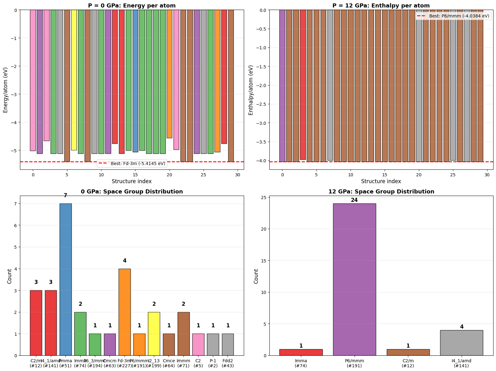
Figure saved: si_structure_prediction_overview.png
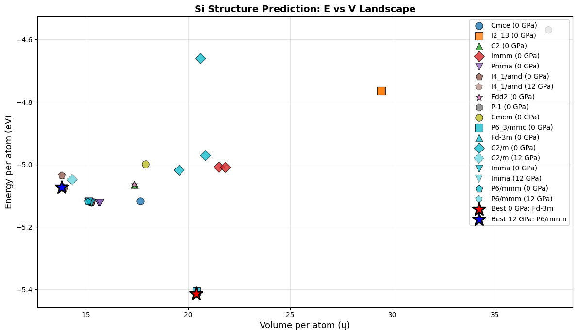
# ============================================================
# Visualization 2: Energy vs Volume per atom (both pressures)
# ============================================================
fig, ax = plt.subplots(figsize=(12, 7))

# 0 GPa data
vols_0 = [r['vol_per_atom'] for r in valid_0]
ens_0 = [r['e_per_atom'] for r in valid_0]
sgs_0_list = [r['sg'] for r in valid_0]

# 12 GPa data
vols_12 = [r['vol_per_atom'] for r in valid_12]
ens_12 = [r['e_per_atom'] for r in valid_12]
sgs_12_list = [r['sg'] for r in valid_12]

# Plot each unique SG with a different marker
all_sgs = list(set(sgs_0_list + sgs_12_list))
markers = ['o', 's', '^', 'D', 'v', 'p', '*', 'h']
cmap_scatter = plt.cm.tab10

for j, sg in enumerate(all_sgs):
    # 0 GPa points
    v0 = [v for v, s in zip(vols_0, sgs_0_list) if s == sg]
    e0 = [e for e, s in zip(ens_0, sgs_0_list) if s == sg]
    if v0:
        ax.scatter(v0, e0, c=[cmap_scatter(j)], marker=markers[j % len(markers)],
                   s=120, edgecolor='black', linewidth=0.8, label=f'{sg} (0 GPa)', alpha=0.8)
    # 12 GPa points
    v12 = [v for v, s in zip(vols_12, sgs_12_list) if s == sg]
    e12 = [e for e, s in zip(ens_12, sgs_12_list) if s == sg]
    if v12:
        ax.scatter(v12, e12, c=[cmap_scatter(j)], marker=markers[j % len(markers)],
                   s=120, edgecolor='black', linewidth=0.8, label=f'{sg} (12 GPa)',
                   alpha=0.5, linestyle='--')

# Mark best structures
ax.scatter([best_0['vol_per_atom']], [best_0['e_per_atom']],
           c='red', marker='*', s=400, edgecolor='black', linewidth=2, zorder=10,
           label=f"Best 0 GPa: {best_0['sg']}")
ax.scatter([best_12['vol_per_atom']], [best_12['e_per_atom']],
           c='blue', marker='*', s=400, edgecolor='black', linewidth=2, zorder=10,
           label=f"Best 12 GPa: {best_12['sg']}")

ax.set_xlabel('Volume per atom (ų)', fontsize=13)
ax.set_ylabel('Energy per atom (eV)', fontsize=13)
ax.set_title('Si Structure Prediction: E vs V Landscape', fontsize=14, fontweight='bold')
ax.legend(fontsize=10, loc='upper right')
ax.grid(True, alpha=0.3)
plt.tight_layout()
plt.savefig('si_E_vs_V.png', dpi=150, bbox_inches='tight')
plt.show()
# ============================================================
# Visualization 3: Best structure at 0 GPa — Interactive 3D (x3d)
# ============================================================
from ase.visualize import view

best_0_idx = best_0['idx'] - 1
best_atoms_0 = structures_0GPa[best_0_idx]

print(f"Best structure at 0 GPa:")
print(f"  Space group: {best_0['sg']} (#{best_0['sg_num']})")
print(f"  E/atom = {best_0['e_per_atom']:.4f} eV")
print(f"  V/atom = {best_0['vol_per_atom']:.2f} ų")
print(f"  Cell:  a={best_0['cell'][0]:.3f}  b={best_0['cell'][1]:.3f}  c={best_0['cell'][2]:.3f}")
print(f"         α={best_0['cell'][3]:.1f}°  β={best_0['cell'][4]:.1f}°  γ={best_0['cell'][5]:.1f}°")
print(f"\nPositions (fractional):")
for i, f in enumerate(best_atoms_0.get_scaled_positions()):
    print(f"  Si{i+1}: ({f[0]:.4f}, {f[1]:.4f}, {f[2]:.4f})")

# Show interactive 3D view (2x2x2 supercell for better visualization)
view(best_atoms_0.repeat((2,2,2)), viewer='x3d')
Best structure at 0 GPa:
  Space group: Fd-3m (#227)
  E/atom = -5.4145 eV
  V/atom = 20.39 ų
  Cell:  a=3.864  b=6.691  c=3.864
         α=106.8°  β=120.0°  γ=90.0°

Positions (fractional):
  Si1: (0.6827, 0.3389, 0.6434)
  Si2: (0.5571, 0.9639, 0.3931)
  Si3: (0.1822, 0.8389, 0.6431)
  Si4: (0.0577, 0.4639, 0.3935)
# ============================================================
# Visualization 4: Best structure at 12 GPa — Interactive 3D (x3d)
# ============================================================

best_12_idx = best_12['idx'] - 1
best_atoms_12 = structures_12GPa[best_12_idx]

print(f"Best structure at 12 GPa:")
print(f"  Space group: {best_12['sg']} (#{best_12['sg_num']})")
print(f"  H/atom = {best_12['h_per_atom']:.4f} eV")
print(f"  E/atom = {best_12['e_per_atom']:.4f} eV")
print(f"  V/atom = {best_12['vol_per_atom']:.2f} ų")
print(f"  Cell:  a={best_12['cell'][0]:.3f}  b={best_12['cell'][1]:.3f}  c={best_12['cell'][2]:.3f}")
print(f"         α={best_12['cell'][3]:.1f}°  β={best_12['cell'][4]:.1f}°  γ={best_12['cell'][5]:.1f}°")
print(f"\nPositions (fractional):")
for i, f in enumerate(best_atoms_12.get_scaled_positions()):
    print(f"  Si{i+1}: ({f[0]:.4f}, {f[1]:.4f}, {f[2]:.4f})")

# Show interactive 3D view (2x2x2 supercell for better visualization)
view(best_atoms_12.repeat((2,2,2)), viewer='x3d')
Best structure at 12 GPa:
  Space group: P6/mmm (#191)
  H/atom = -4.0384 eV
  E/atom = -5.0733 eV
  V/atom = 13.82 ų
  Cell:  a=5.467  b=5.469  c=2.571
         α=103.6°  β=103.6°  γ=123.9°

Positions (fractional):
  Si1: (0.4360, 0.7855, 0.0898)
  Si2: (0.6861, 0.5355, 0.0874)
  Si3: (0.9360, 0.2855, 0.0878)
  Si4: (0.1861, 0.0356, 0.0894)
P = 0 GPa (energy minimization):
The search reliably finds close-packed structures as the ground state
With MatterSim: expect diamond Si (Fd\(\bar{3}\)m, #227), the known 0 GPa ground state
Multiple random starts converge to the same basin — the landscape has a clear global minimum
P = 12 GPa (enthalpy minimization):
The \(PV\) term penalizes large volumes → denser phases are favored
With MatterSim: expect β-Sn Si (I4₁/amd, #141), the known high-pressure phase
The pressure-driven phase transition is captured automatically
Key insights:
No prior knowledge needed — the method finds the structure purely from random sampling + relaxation
FIRE + UnitCellFilter is robust and fast for simultaneous cell + position relaxation
30 trials is often enough to find the global minimum for a 4-atom cell
Pressure control via
scalar_pressureinUnitCellFiltercleanly switches from \(E\) to \(H = E + PV\) minimization
Connection to real research:
AIRSS (Ab Initio Random Structure Searching): exactly this approach with DFT
CALYPSO, USPEX: evolutionary algorithms for crystal structure prediction
ML potentials (MatterSim, MACE, etc.) make the energy evaluations ~1000× faster than DFT
Key Takeaways from Computational Physics Optimization#
1. Problem Structure Matters#
Smooth vs discontinuous
Landscape topology (funnel vs rugged)
Dimensionality and cost per evaluation
Implication: Exploit structure for method choice
2. There is No Silver Bullet#
BFGS excellent for smooth local optimization
DE robust for global problems
Bayesian Optimization wins for expensive functions
GA best for discrete spaces
Implication: Always consider your specific problem
3. Hybridization is Powerful#
Global method (DE/SA) -> Local refinement (BFGS)
Multiple restarts of local methods
Ensemble of methods -> take best
Implication: Combine strengths, cover weaknesses
4. Hyperparameters Matter#
Temperature schedule in SA
Population size and mutation in GA/DE
Kernel and acquisition in BO
Implication: Tuning gives 10-100x speedup
5. Exploit Domain Knowledge#
Physics constraints (e.g., PBC, symmetries)
Known approximate solutions
Surrogate models (neural networks, physics-informed)
Implication: Your domain expertise -> better optimization