Lecture 20 — Machine Learning I

Foundations & Classical Methods

Computational Physics — Spring 2026

From Curve Fitting to Machine Learning

In Lecture 7 you learned to fit a model \(f(x; \boldsymbol{\theta})\) to data by minimising the sum of squared residuals:

\[ \min_{\boldsymbol{\theta}} \sum_{i=1}^{N} \bigl[y_i - f(x_i;\boldsymbol{\theta})\bigr]^2 \]

In Lectures 15-19 you studied many optimisation algorithms to solve exactly this kind of problem.

Machine learning is the same idea, scaled up:

Curve Fitting (Lecture 7)	Machine Learning
Choose a functional form	Choose a model architecture
Minimise residuals	Minimise a loss function
Use least squares / curve_fit	Use gradient descent (Lecture 15)
A few parameters	Hundreds to billions of parameters
Works on small data	Needs more data as model grows

The key new idea: generalisation — we care how the model performs on unseen data, not just the data it was trained on.

import numpy as np
import matplotlib.pyplot as plt
from sklearn.model_selection import train_test_split

plt.rcParams['figure.figsize'] = [6, 4]
plt.rcParams['font.size'] = 9

print("Ready for Machine Learning!")

Ready for Machine Learning!

I. The Machine-Learning Framework

Supervised vs Unsupervised Learning

Type	Input	Goal	Example
Supervised	\((\mathbf{x}_i, y_i)\) pairs	Predict \(y\) from \(\mathbf{x}\)	Predict energy from atomic positions
Unsupervised	\(\mathbf{x}_i\) only	Find structure	Cluster crystal structures

Within supervised learning:

• Regression: \(y\) is continuous (e.g. energy, temperature)

• Classification: \(y\) is a discrete label (e.g. phase = ordered / disordered)

Training, Validation, and Test Sets

The most important principle in ML: never evaluate your model on data it was trained on.

We split the data:

Full Dataset
├── Training set   (70-80%)  → fit the model
├── Validation set  (10-15%) → tune hyperparameters
└── Test set        (10-15%) → final evaluation (touch ONCE)

For small datasets, k-fold cross-validation is more efficient: split data into \(k\) folds, train on \(k-1\), validate on the remaining one, rotate, and average the scores.

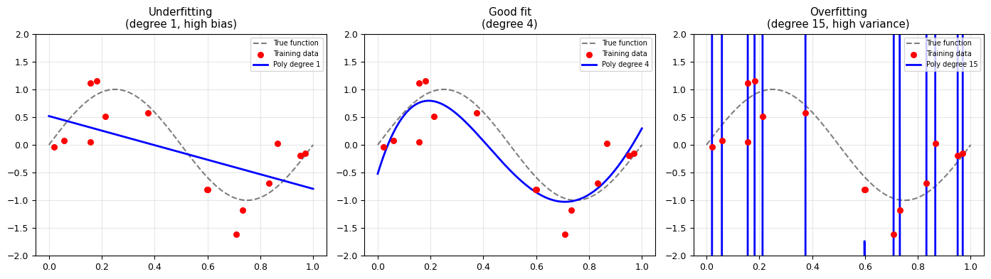
The Bias–Variance Trade-off

For any model, the expected prediction error decomposes as:

\[ \text{Error} = \text{Bias}^2 + \text{Variance} + \text{Irreducible noise} \]

• Bias = error from wrong assumptions (model too simple → underfitting)

• Variance = error from sensitivity to training data (model too complex → overfitting)

The sweet spot is in the middle — complex enough to capture the real pattern, simple enough to generalise.

# Demo: Overfitting vs Underfitting with polynomial regression
np.random.seed(42)

# True function: a simple curve
x_true = np.linspace(0, 1, 200)
y_true = np.sin(2 * np.pi * x_true)

# Noisy training data (only 15 points)
N_train = 15
x_train = np.sort(np.random.rand(N_train))
y_train = np.sin(2 * np.pi * x_train) + 0.3 * np.random.randn(N_train)

fig, axes = plt.subplots(1, 3, figsize=(14, 4))
degrees = [1, 4, 15]
titles = ['Underfitting\n(degree 1, high bias)',
          'Good fit\n(degree 4)',
          'Overfitting\n(degree 15, high variance)']

for ax, deg, title in zip(axes, degrees, titles):
    # Fit polynomial
    coeffs = np.polyfit(x_train, y_train, deg)
    y_fit = np.polyval(coeffs, x_true)

    ax.plot(x_true, y_true, 'k--', alpha=0.5, label='True function')
    ax.scatter(x_train, y_train, c='red', s=30, zorder=5, label='Training data')
    ax.plot(x_true, y_fit, 'b-', lw=2, label=f'Poly degree {deg}')
    ax.set_ylim(-2, 2)
    ax.set_title(title)
    ax.legend(fontsize=7)
    ax.grid(alpha=0.3)

plt.tight_layout()
plt.show()

/var/folders/21/r088s2vn77n_bgl39f24mdfm0000gn/T/ipykernel_87566/1047291385.py:21: RankWarning: Polyfit may be poorly conditioned
  coeffs = np.polyfit(x_train, y_train, deg)

II. Linear & Logistic Regression — Revisited

Linear Regression (Regression)

You already know this from Lecture 7! Given features \(\mathbf{X}\) and targets \(\mathbf{y}\), find weights \(\mathbf{w}\) that minimise:

\[ L(\mathbf{w}) = \|\mathbf{y} - \mathbf{X}\mathbf{w}\|^2 \]

Closed-form solution (normal equation): \(\mathbf{w} = (\mathbf{X}^T \mathbf{X})^{-1} \mathbf{X}^T \mathbf{y}\)

The ML addition: regularisation to prevent overfitting:

• Ridge (L2): \(L = \|\mathbf{y} - \mathbf{X}\mathbf{w}\|^2 + \alpha\|\mathbf{w}\|^2\) — shrinks weights

• Lasso (L1): \(L = \|\mathbf{y} - \mathbf{X}\mathbf{w}\|^2 + \alpha\|\mathbf{w}\|_1\) — makes weights sparse

from sklearn.linear_model import LinearRegression, Ridge, Lasso
from sklearn.preprocessing import PolynomialFeatures
from sklearn.pipeline import make_pipeline
from sklearn.metrics import mean_squared_error

# Same data as above — fit degree-15 polynomial WITH regularisation
fig, axes = plt.subplots(1, 3, figsize=(14, 4))

models = [
    ('No regularisation', make_pipeline(PolynomialFeatures(15), LinearRegression())),
    ('Ridge (L2)', make_pipeline(PolynomialFeatures(15), Ridge(alpha=0.01))),
    ('Lasso (L1)', make_pipeline(PolynomialFeatures(15), Lasso(alpha=0.01, max_iter=5000))),
]

for ax, (name, model) in zip(axes, models):
    model.fit(x_train.reshape(-1, 1), y_train)
    y_pred = model.predict(x_true.reshape(-1, 1))

    ax.plot(x_true, y_true, 'k--', alpha=0.5, label='True')
    ax.scatter(x_train, y_train, c='red', s=30, zorder=5)
    ax.plot(x_true, y_pred, 'b-', lw=2)
    ax.set_ylim(-2, 2)
    ax.set_title(name)
    ax.grid(alpha=0.3)

plt.tight_layout()
plt.show()
print("Regularisation tames the overfitting of a degree-15 polynomial!")

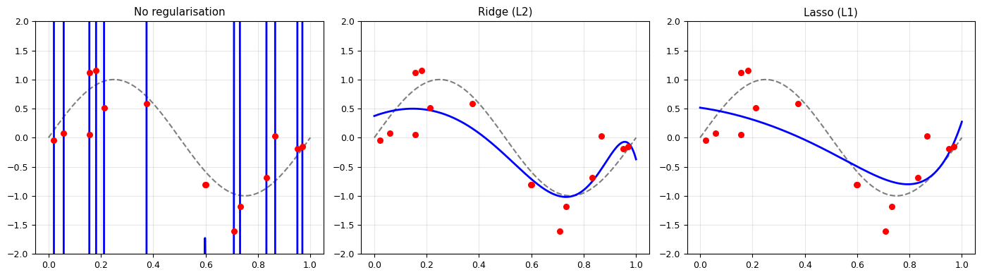
Regularisation tames the overfitting of a degree-15 polynomial!

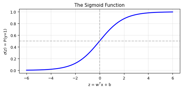
Logistic Regression (Classification)

For binary classification (\(y \in \{0, 1\}\)), we model the probability:

\[ P(y=1 \mid \mathbf{x}) = \sigma(\mathbf{w}^T \mathbf{x} + b) = \frac{1}{1 + e^{-(\mathbf{w}^T \mathbf{x} + b)}} \]

where \(\sigma\) is the sigmoid (logistic) function.

The loss function is the cross-entropy:

\[ L = -\sum_i \bigl[ y_i \log \hat{y}_i + (1-y_i) \log(1-\hat{y}_i) \bigr] \]

No closed-form solution — we use gradient descent (Lecture 15!).

# The sigmoid function
z = np.linspace(-6, 6, 200)
sigmoid = 1 / (1 + np.exp(-z))

plt.figure(figsize=(6, 3))
plt.plot(z, sigmoid, 'b-', lw=2)
plt.axhline(0.5, color='gray', ls='--', alpha=0.5)
plt.axvline(0, color='gray', ls='--', alpha=0.5)
plt.xlabel('z = w$^T$x + b')
plt.ylabel('$\\sigma(z)$ = P(y=1)')
plt.title('The Sigmoid Function')
plt.grid(alpha=0.3)
plt.tight_layout()
plt.show()

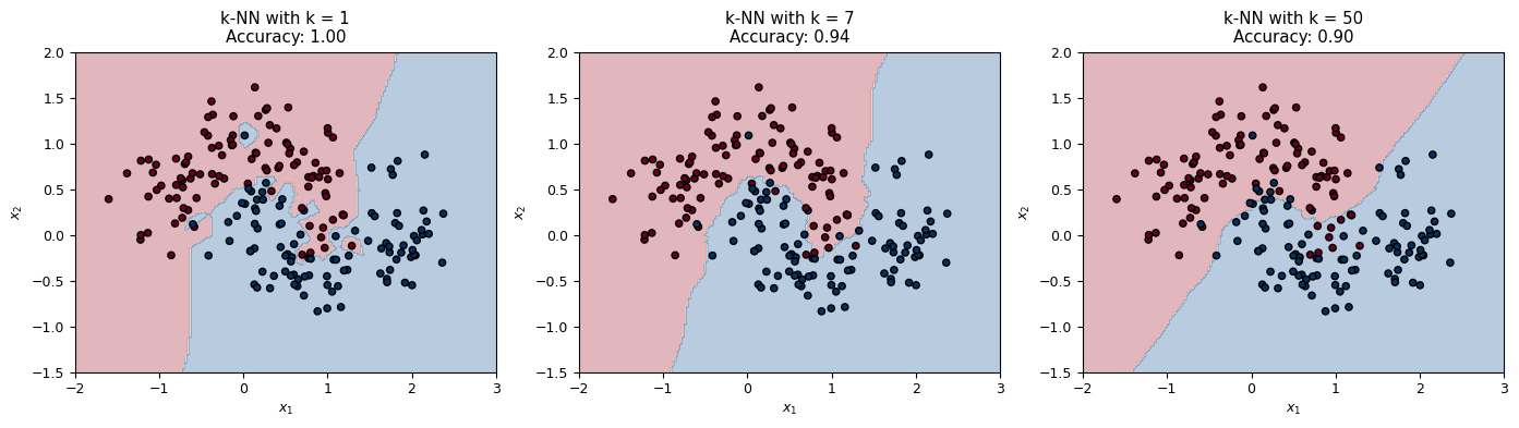
III. k-Nearest Neighbours (k-NN)

The simplest ML algorithm: to predict the label of a new point \(\mathbf{x}\),

1. Find the \(k\) closest training points (by Euclidean distance).

2. Classification: majority vote among the \(k\) neighbours.

3. Regression: average of the \(k\) neighbours’ values.

Hyperparameter: \(k\)

• Small \(k\) → complex boundary (overfitting)

• Large \(k\) → smoother boundary (underfitting)

Pros: Simple, no training phase, works well for small datasets
Cons: Slow at prediction time (\(O(Nd)\) per query), sensitive to irrelevant features

from sklearn.datasets import make_moons
from sklearn.neighbors import KNeighborsClassifier

# Generate a toy 2-class dataset
X_moons, y_moons = make_moons(n_samples=200, noise=0.25, random_state=42)

fig, axes = plt.subplots(1, 3, figsize=(14, 4))

for ax, k in zip(axes, [1, 7, 50]):
    clf = KNeighborsClassifier(n_neighbors=k)
    clf.fit(X_moons, y_moons)

    # Decision boundary
    xx, yy = np.meshgrid(np.linspace(-2, 3, 200), np.linspace(-1.5, 2, 200))
    Z = clf.predict(np.c_[xx.ravel(), yy.ravel()]).reshape(xx.shape)

    ax.contourf(xx, yy, Z, alpha=0.3, cmap='RdBu')
    ax.scatter(X_moons[:, 0], X_moons[:, 1], c=y_moons, cmap='RdBu',
               edgecolors='k', s=20)
    ax.set_title(f'k-NN with k = {k}\nAccuracy: {clf.score(X_moons, y_moons):.2f}')
    ax.set_xlabel('$x_1$'); ax.set_ylabel('$x_2$')

plt.tight_layout()
plt.show()

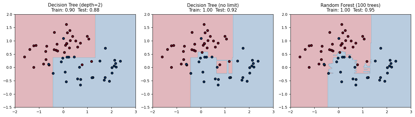
IV. Decision Trees & Random Forests

Decision Trees

A decision tree splits the feature space with axis-aligned cuts:

           Is x₁ > 0.5?
          /             \
       Yes               No
    Is x₂ > 0.3?      Class B
    /          \
Class A     Class B

At each node, the algorithm picks the feature and threshold that best separates the classes (measured by Gini impurity or information gain).

Pros: Interpretable, handles mixed feature types
Cons: Overfits easily (high variance), unstable (small data changes → different tree)

Random Forests: Wisdom of the Crowd

A random forest fixes the overfitting problem by training many trees on random subsets of the data and features, then averaging their predictions.

This is an example of ensemble learning — combining weak learners into a strong one.

Each tree:

1. Gets a random bootstrap sample of the training data

2. At each split, considers only a random subset of features

3. Grows to full depth (overfits individually)

The ensemble averages out individual errors → low bias AND low variance.

from sklearn.tree import DecisionTreeClassifier
from sklearn.ensemble import RandomForestClassifier

fig, axes = plt.subplots(1, 3, figsize=(14, 4))

classifiers = [
    ('Decision Tree (depth=2)', DecisionTreeClassifier(max_depth=2, random_state=42)),
    ('Decision Tree (no limit)', DecisionTreeClassifier(random_state=42)),
    ('Random Forest (100 trees)', RandomForestClassifier(n_estimators=100, random_state=42)),
]

X_train_m, X_test_m, y_train_m, y_test_m = train_test_split(
    X_moons, y_moons, test_size=0.3, random_state=42)

for ax, (name, clf) in zip(axes, classifiers):
    clf.fit(X_train_m, y_train_m)

    xx, yy = np.meshgrid(np.linspace(-2, 3, 200), np.linspace(-1.5, 2, 200))
    Z = clf.predict(np.c_[xx.ravel(), yy.ravel()]).reshape(xx.shape)

    ax.contourf(xx, yy, Z, alpha=0.3, cmap='RdBu')
    ax.scatter(X_test_m[:, 0], X_test_m[:, 1], c=y_test_m, cmap='RdBu',
               edgecolors='k', s=30)
    train_acc = clf.score(X_train_m, y_train_m)
    test_acc = clf.score(X_test_m, y_test_m)
    ax.set_title(f'{name}\nTrain: {train_acc:.2f}  Test: {test_acc:.2f}')

plt.tight_layout()
plt.show()

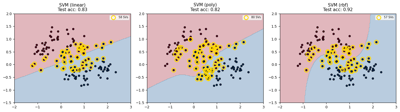
V. Support Vector Machines (SVM)

SVM finds the maximum-margin hyperplane that separates two classes.

For linearly separable data, SVM solves:

\[ \min_{\mathbf{w}, b} \frac{1}{2}\|\mathbf{w}\|^2 \quad \text{s.t.} \quad y_i(\mathbf{w}^T \mathbf{x}_i + b) \geq 1 \;\;\forall i \]

The Kernel Trick

For non-linear boundaries, SVM maps data to a higher-dimensional space using a kernel function \(K(\mathbf{x}_i, \mathbf{x}_j)\):

Kernel	Formula	Use case
Linear	\(\mathbf{x}_i^T \mathbf{x}_j\)	Linearly separable
Polynomial	\((\mathbf{x}_i^T \mathbf{x}_j + c)^d\)	Moderate non-linearity
RBF (Gaussian)	\(\exp(-\gamma|\mathbf{x}_i - \mathbf{x}_j|^2)\)	Most common default

The key insight: the algorithm only needs dot products between data points, so we never explicitly compute the high-dimensional mapping.

from sklearn.svm import SVC

fig, axes = plt.subplots(1, 3, figsize=(14, 4))

kernels = ['linear', 'poly', 'rbf']
for ax, kernel in zip(axes, kernels):
    clf = SVC(kernel=kernel, gamma='auto', random_state=42)
    clf.fit(X_train_m, y_train_m)

    xx, yy = np.meshgrid(np.linspace(-2, 3, 200), np.linspace(-1.5, 2, 200))
    Z = clf.predict(np.c_[xx.ravel(), yy.ravel()]).reshape(xx.shape)

    ax.contourf(xx, yy, Z, alpha=0.3, cmap='RdBu')
    ax.scatter(X_train_m[:, 0], X_train_m[:, 1], c=y_train_m, cmap='RdBu',
               edgecolors='k', s=20)
    # Highlight support vectors
    ax.scatter(clf.support_vectors_[:, 0], clf.support_vectors_[:, 1],
               s=100, facecolors='none', edgecolors='gold', lw=2,
               label=f'{len(clf.support_vectors_)} SVs')
    test_acc = clf.score(X_test_m, y_test_m)
    ax.set_title(f'SVM ({kernel})\nTest acc: {test_acc:.2f}')
    ax.legend(fontsize=7)

plt.tight_layout()
plt.show()

VI. The scikit-learn Workflow

Every scikit-learn model follows the same API:

from sklearn.some_module import SomeModel

## 1. Create the model with hyperparameters
model = SomeModel(hyperparam1=value1, ...)

## 2. Fit to training data
model.fit(X_train, y_train)

## 3. Predict on new data
y_pred = model.predict(X_test)

## 4. Evaluate
score = model.score(X_test, y_test)

This uniform interface makes it trivial to swap models and compare.

Model Comparison on the Moons Dataset

from sklearn.linear_model import LogisticRegression

models = {
    'Logistic Regression': LogisticRegression(),
    'k-NN (k=5)': KNeighborsClassifier(n_neighbors=5),
    'Decision Tree': DecisionTreeClassifier(max_depth=5, random_state=42),
    'Random Forest': RandomForestClassifier(n_estimators=100, random_state=42),
    'SVM (RBF)': SVC(kernel='rbf', random_state=42),
}

print(f"{'Model':<25} {'Train Acc':>10} {'Test Acc':>10}")
print('-' * 47)
for name, model in models.items():
    model.fit(X_train_m, y_train_m)
    train_acc = model.score(X_train_m, y_train_m)
    test_acc = model.score(X_test_m, y_test_m)
    print(f"{name:<25} {train_acc:>10.3f} {test_acc:>10.3f}")

Model                      Train Acc   Test Acc
-----------------------------------------------
Logistic Regression            0.836      0.850
k-NN (k=5)                     0.950      0.933
Decision Tree                  0.986      0.917
Random Forest                  1.000      0.950
SVM (RBF)                      0.936      0.933

Cross-Validation: More Reliable Evaluation

from sklearn.model_selection import cross_val_score

print(f"{'Model':<25} {'CV Accuracy (mean +/- std)':>30}")
print('-' * 57)
for name, model in models.items():
    scores = cross_val_score(model, X_moons, y_moons, cv=5, scoring='accuracy')
    print(f"{name:<25} {scores.mean():>10.3f} +/- {scores.std():.3f}")

Model                         CV Accuracy (mean +/- std)
---------------------------------------------------------
Logistic Regression            0.845 +/- 0.033
k-NN (k=5)                     0.940 +/- 0.041
Decision Tree                  0.905 +/- 0.048
Random Forest                  0.940 +/- 0.037
SVM (RBF)                      0.940 +/- 0.025

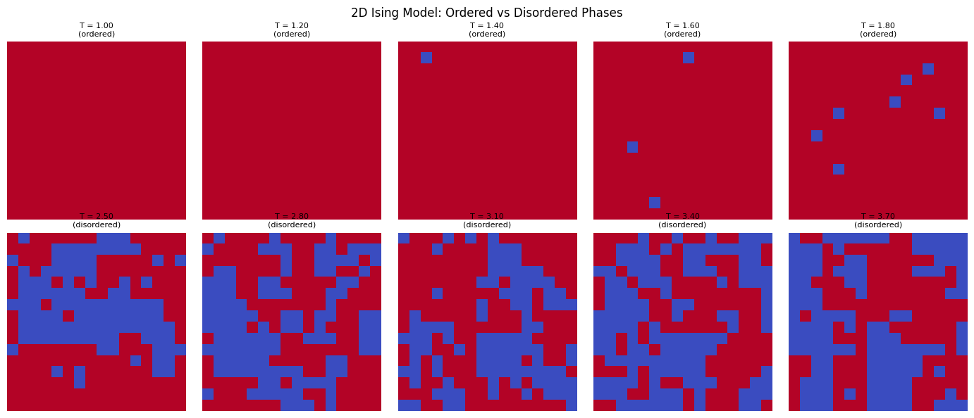
VII. Physics Application: Classifying Ising Model Phases

The 2D Ising model is a lattice of spins \(s_i \in \{-1, +1\}\) with nearest-neighbour interactions:

\[ H = -J \sum_{\langle i,j \rangle} s_i s_j \]

It undergoes a phase transition at the critical temperature \(T_c \approx 2.269\,J/k_B\):

• \(T < T_c\): ordered (ferromagnetic) phase — most spins aligned

• \(T > T_c\): disordered (paramagnetic) phase — spins random

Question: Can ML learn to distinguish the two phases directly from spin configurations, without being told about \(T_c\)?

We will:

1. Generate Ising configurations at various temperatures using Monte Carlo

2. Label them: ordered (\(T < T_c\)) vs disordered (\(T > T_c\))

3. Train classifiers on the raw spin configurations

4. See which models learn the phase boundary

Step 1: Generate Ising Configurations via Metropolis Algorithm

We use the Metropolis algorithm from Lecture 14 to sample spin configurations at different temperatures.

def metropolis_ising(L, T, n_sweeps=1000, n_equil=500):
    """
    Metropolis Monte Carlo for the 2D Ising model on an L x L lattice.
    Returns spin configurations sampled after equilibration.

    Parameters
    ----------
    L : int — lattice size
    T : float — temperature (in units of J/k_B)
    n_sweeps : int — total MC sweeps
    n_equil : int — equilibration sweeps (discarded)

    Returns
    -------
    configs : list of (L, L) arrays — sampled spin configurations
    """
    # Initialise random spin configuration
    spins = np.random.choice([-1, 1], size=(L, L))
    beta = 1.0 / T
    configs = []

    for sweep in range(n_sweeps):
        for _ in range(L * L):
            # Pick a random spin
            i, j = np.random.randint(0, L, size=2)
            # Compute energy change for flipping spin (i, j)
            neighbours = (
                spins[(i+1) % L, j] + spins[(i-1) % L, j] +
                spins[i, (j+1) % L] + spins[i, (j-1) % L]
            )
            dE = 2 * spins[i, j] * neighbours
            # Metropolis acceptance
            if dE <= 0 or np.random.rand() < np.exp(-beta * dE):
                spins[i, j] *= -1

        # Save configuration every 10 sweeps after equilibration
        if sweep >= n_equil and sweep % 10 == 0:
            configs.append(spins.copy())

    return configs

print("Metropolis sampler ready.")

Metropolis sampler ready.

# Generate training data: spin configurations at various temperatures
L = 16  # 16x16 lattice
T_c = 2.269  # Critical temperature

# Sample temperatures below and above T_c
temperatures = np.concatenate([
    np.linspace(1.0, 2.0, 6),   # ordered phase
    np.linspace(2.5, 4.0, 6),   # disordered phase
])

X_ising = []  # Flattened spin configurations
y_ising = []  # Labels: 0 = ordered, 1 = disordered
T_ising = []  # Temperature (for analysis)

print("Generating Ising configurations...")
for T in temperatures:
    configs = metropolis_ising(L, T, n_sweeps=2000, n_equil=1000)
    for cfg in configs:
        X_ising.append(cfg.flatten())
        y_ising.append(0 if T < T_c else 1)
        T_ising.append(T)
    print(f"  T = {T:.2f}: {len(configs)} configurations")

X_ising = np.array(X_ising)
y_ising = np.array(y_ising)
T_ising = np.array(T_ising)

print(f"\nTotal dataset: {len(X_ising)} configurations of size {L}x{L} = {L*L} features")
print(f"Ordered: {np.sum(y_ising == 0)}, Disordered: {np.sum(y_ising == 1)}")

Generating Ising configurations...
  T = 1.00: 100 configurations
  T = 1.20: 100 configurations
  T = 1.40: 100 configurations
  T = 1.60: 100 configurations
  T = 1.80: 100 configurations
  T = 2.00: 100 configurations
  T = 2.50: 100 configurations
  T = 2.80: 100 configurations
  T = 3.10: 100 configurations
  T = 3.40: 100 configurations
  T = 3.70: 100 configurations
  T = 4.00: 100 configurations

Total dataset: 1200 configurations of size 16x16 = 256 features
Ordered: 600, Disordered: 600

# Visualise some configurations
fig, axes = plt.subplots(2, 5, figsize=(14, 6))

for i, T in enumerate(temperatures[:5]):
    idx = np.where(np.isclose(T_ising, T))[0][0]
    axes[0, i].imshow(X_ising[idx].reshape(L, L), cmap='coolwarm', vmin=-1, vmax=1)
    axes[0, i].set_title(f'T = {T:.2f}\n(ordered)', fontsize=8)
    axes[0, i].axis('off')

for i, T in enumerate(temperatures[6:11]):
    idx = np.where(np.isclose(T_ising, T))[0][0]
    axes[1, i].imshow(X_ising[idx].reshape(L, L), cmap='coolwarm', vmin=-1, vmax=1)
    axes[1, i].set_title(f'T = {T:.2f}\n(disordered)', fontsize=8)
    axes[1, i].axis('off')

plt.suptitle('2D Ising Model: Ordered vs Disordered Phases', fontsize=12)
plt.tight_layout()
plt.show()

Step 2: Train Classifiers on Spin Configurations

# Split into training and test sets
X_train_I, X_test_I, y_train_I, y_test_I, T_train_I, T_test_I = train_test_split(
    X_ising, y_ising, T_ising, test_size=0.3, random_state=42, stratify=y_ising
)

print(f"Training set: {len(X_train_I)} samples")
print(f"Test set:     {len(X_test_I)} samples")

Training set: 840 samples
Test set:     360 samples

# Train multiple classifiers
ising_models = {
    'Logistic Regression': LogisticRegression(max_iter=1000),
    'k-NN (k=5)': KNeighborsClassifier(n_neighbors=5),
    'Random Forest': RandomForestClassifier(n_estimators=100, random_state=42),
    'SVM (RBF)': SVC(kernel='rbf', probability=True, random_state=42),
}

print(f"{'Model':<25} {'Train Acc':>10} {'Test Acc':>10}")
print('-' * 47)

trained_models = {}
for name, model in ising_models.items():
    model.fit(X_train_I, y_train_I)
    train_acc = model.score(X_train_I, y_train_I)
    test_acc = model.score(X_test_I, y_test_I)
    print(f"{name:<25} {train_acc:>10.3f} {test_acc:>10.3f}")
    trained_models[name] = model

Model                      Train Acc   Test Acc
-----------------------------------------------
Logistic Regression            0.883      0.667
k-NN (k=5)                     0.854      0.797
Random Forest                  1.000      0.992
SVM (RBF)                      1.000      0.997

Step 3: Test Near the Phase Transition

The real test: how do our classifiers perform at temperatures near \(T_c\), where the phase distinction is subtle?

# Generate test configurations near the critical temperature
T_critical_test = np.linspace(1.5, 3.5, 20)

print("Generating critical-region test data...")
X_crit = []
T_crit = []
for T in T_critical_test:
    configs = metropolis_ising(L, T, n_sweeps=1500, n_equil=800)
    for cfg in configs:
        X_crit.append(cfg.flatten())
        T_crit.append(T)

X_crit = np.array(X_crit)
T_crit = np.array(T_crit)
print(f"Generated {len(X_crit)} test configurations.")

Generating critical-region test data...
Generated 1400 test configurations.

# Plot P(disordered) vs temperature for each model
fig, ax = plt.subplots(figsize=(8, 5))

colors = ['blue', 'green', 'orange', 'red']
for (name, model), color in zip(trained_models.items(), colors):
    # Get probability of being "disordered" for each temperature
    probs = []
    for T in T_critical_test:
        mask = np.isclose(T_crit, T)
        if hasattr(model, 'predict_proba'):
            p = model.predict_proba(X_crit[mask])[:, 1].mean()
        else:
            p = model.predict(X_crit[mask]).mean()
        probs.append(p)
    ax.plot(T_critical_test, probs, 'o-', color=color, label=name, lw=2)

ax.axvline(T_c, color='black', ls='--', lw=2, label=f'$T_c$ = {T_c:.3f}')
ax.set_xlabel('Temperature $T$ ($J/k_B$)', fontsize=11)
ax.set_ylabel('P(disordered)', fontsize=11)
ax.set_title('ML Phase Classification of the 2D Ising Model', fontsize=12)
ax.legend(fontsize=9)
ax.grid(alpha=0.3)
plt.tight_layout()
plt.show()

print("All models learn a sharp transition near the true T_c!")

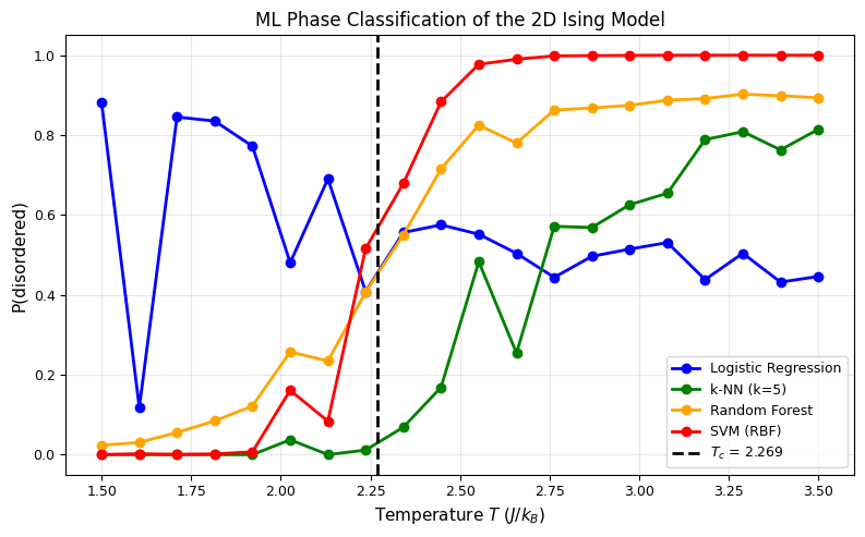
All models learn a sharp transition near the true T_c!

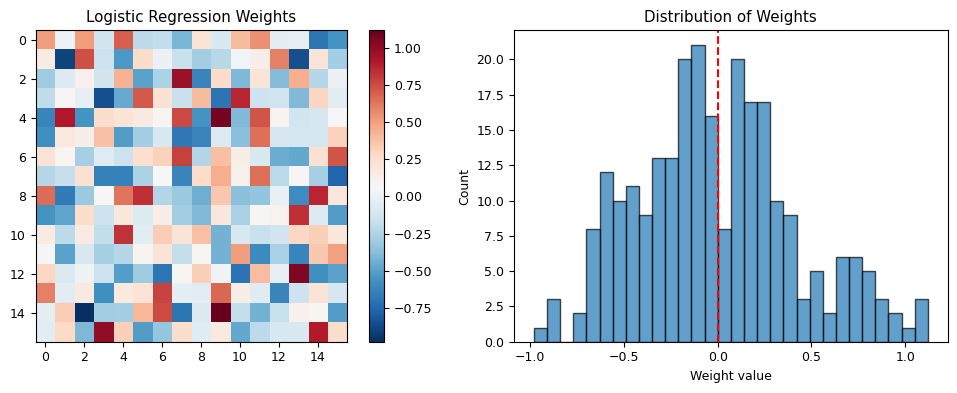
What Did Logistic Regression Learn?

Logistic regression only achieved ~67% accuracy — barely better than random. Why? Since it is a linear model, we can inspect its weights to find out. Each weight corresponds to one spin site.

# Visualise the logistic regression weights
lr_model = trained_models['Logistic Regression']
weights = lr_model.coef_[0].reshape(L, L)

fig, axes = plt.subplots(1, 2, figsize=(10, 4))

im = axes[0].imshow(weights, cmap='RdBu_r')
axes[0].set_title('Logistic Regression Weights')
plt.colorbar(im, ax=axes[0])

axes[1].hist(weights.flatten(), bins=30, edgecolor='black', alpha=0.7)
axes[1].set_xlabel('Weight value')
axes[1].set_ylabel('Count')
axes[1].set_title('Distribution of Weights')
axes[1].axvline(0, color='red', ls='--')

plt.tight_layout()
plt.show()

print(f"The weights are roughly uniform — LR learned w^T s + b ≈ mean(s_i) = m.")
print(f"But m is NOT the order parameter — |m| is!")
print(f"Ordered phases can have m ≈ +1 OR m ≈ -1, while disordered has m ≈ 0.")
print(f"A linear classifier cannot separate 'both extremes' from 'the middle'.")
print(f"This explains the poor 67% accuracy — and why physics features (|m|) fix it!")

The weights are roughly uniform — LR learned w^T s + b ≈ mean(s_i) = m.
But m is NOT the order parameter — |m| is!
Ordered phases can have m ≈ +1 OR m ≈ -1, while disordered has m ≈ 0.
A linear classifier cannot separate 'both extremes' from 'the middle'.
This explains the poor 67% accuracy — and why physics features (|m|) fix it!

VIII. Feature Engineering for Physics

The logistic regression failure above teaches an important lesson: the right features matter more than the right algorithm.

Raw spin configurations have \(L^2 = 256\) features. A physicist knows that the order parameter is \(|m|\), not \(m\) — and LR can’t compute absolute values. Let’s give the models physics-informed features:

1. Raw features: All \(L^2\) spins (what we did above)

2. Engineered features: \(|m|\), \(m^2\), energy \(E/N\), nearest-neighbour correlation

def extract_physics_features(configs, L):
    """Extract physically meaningful features from spin configurations."""
    features = []
    for cfg_flat in configs:
        cfg = cfg_flat.reshape(L, L)

        # Magnetisation per spin
        m = np.mean(cfg)
        abs_m = np.abs(m)

        # Energy per spin (nearest-neighbour)
        E = 0
        for i in range(L):
            for j in range(L):
                E -= cfg[i, j] * (cfg[(i+1)%L, j] + cfg[i, (j+1)%L])
        E /= L * L

        # Nearest-neighbour correlation
        nn_corr = 0
        for i in range(L):
            for j in range(L):
                nn_corr += cfg[i, j] * cfg[(i+1)%L, j]
        nn_corr /= L * L

        features.append([abs_m, m**2, E, nn_corr])

    return np.array(features)

# Extract physics features
X_phys_train = extract_physics_features(X_train_I, L)
X_phys_test = extract_physics_features(X_test_I, L)

print("Physics features: |m|, m², E/N, <s_i s_j>")
print(f"Shape: {X_phys_train.shape} (only 4 features instead of {L*L}!)")

# Compare: raw features vs physics features
print(f"\n{'Model':<25} {'Raw (256 feat)':>15} {'Physics (4 feat)':>17}")
print('-' * 59)
for name in ['Logistic Regression', 'Random Forest', 'SVM (RBF)']:
    # Raw features
    m1 = ising_models[name].__class__(**ising_models[name].get_params())
    if name == 'Logistic Regression':
        m1.set_params(max_iter=1000)
    m1.fit(X_train_I, y_train_I)
    raw_acc = m1.score(X_test_I, y_test_I)

    # Physics features
    m2 = ising_models[name].__class__(**ising_models[name].get_params())
    if name == 'Logistic Regression':
        m2.set_params(max_iter=1000)
    m2.fit(X_phys_train, y_train_I)
    phys_acc = m2.score(X_phys_test, y_test_I)

    print(f"{name:<25} {raw_acc:>15.3f} {phys_acc:>17.3f}")

print("\nPhysics features work just as well (or better) with 4 features instead of 256!")
print("Domain knowledge is a powerful form of regularisation.")

Physics features: |m|, m², E/N, <s_i s_j>
Shape: (840, 4) (only 4 features instead of 256!)

Model                      Raw (256 feat)  Physics (4 feat)
-----------------------------------------------------------
Logistic Regression                 0.667             1.000
Random Forest                       0.992             1.000
SVM (RBF)                           0.997             1.000

Physics features work just as well (or better) with 4 features instead of 256!
Domain knowledge is a powerful form of regularisation.

IX. Unsupervised Learning: PCA

What if we don’t know the labels? Can we still discover the two phases?

Principal Component Analysis (PCA) finds the directions of maximum variance in the data. If the two phases are truly different, PCA should separate them — without any labels.

from sklearn.decomposition import PCA

# Apply PCA to all Ising configurations
pca = PCA(n_components=2)
X_pca = pca.fit_transform(X_ising)

fig, axes = plt.subplots(1, 2, figsize=(12, 5))

# Colour by label
scatter1 = axes[0].scatter(X_pca[:, 0], X_pca[:, 1], c=y_ising, cmap='coolwarm',
                           s=10, alpha=0.7)
axes[0].set_xlabel(f'PC1 ({pca.explained_variance_ratio_[0]:.1%} variance)')
axes[0].set_ylabel(f'PC2 ({pca.explained_variance_ratio_[1]:.1%} variance)')
axes[0].set_title('PCA coloured by phase label')
plt.colorbar(scatter1, ax=axes[0], label='0=ordered, 1=disordered')

# Colour by temperature
scatter2 = axes[1].scatter(X_pca[:, 0], X_pca[:, 1], c=T_ising, cmap='plasma',
                           s=10, alpha=0.7)
axes[1].set_xlabel(f'PC1 ({pca.explained_variance_ratio_[0]:.1%} variance)')
axes[1].set_ylabel(f'PC2 ({pca.explained_variance_ratio_[1]:.1%} variance)')
axes[1].set_title('PCA coloured by temperature')
plt.colorbar(scatter2, ax=axes[1], label='Temperature $T$')

plt.tight_layout()
plt.show()

print("PCA separates the two phases without any labels!")
print("The first principal component captures the phase transition.")

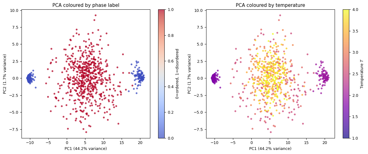
PCA separates the two phases without any labels!
The first principal component captures the phase transition.

Summary

Concept	Key Idea
ML = fitting + generalisation	Same optimisation, but we care about unseen data
Bias–variance trade-off	Simple models underfit, complex models overfit
Regularisation	Penalise complexity (Ridge, Lasso)
k-NN	Classify by nearest neighbours
Decision trees / Random forests	Split features; ensemble reduces variance
SVM	Maximum-margin hyperplane + kernel trick
PCA	Unsupervised dimensionality reduction
Feature engineering	Domain knowledge > more data

Key takeaway: The same Ising phase transition can be detected by supervised classification, unsupervised PCA, or simple physics features. ML is most powerful when combined with physical insight.

Next lecture: We move from classical algorithms to neural networks — models that can learn their own features.